If you want to test values to see if they begin with some given specific characters like “x”, ”y”, or “z”, you can create a formula with COUNTIF and SUM functions to return results.
Table of Contents
EXAMPLE
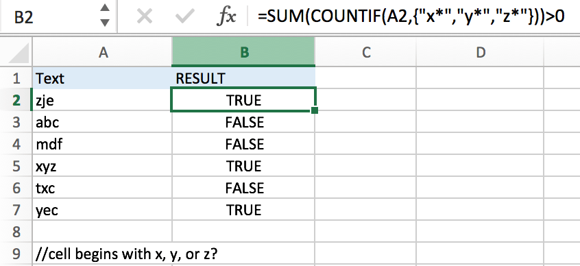
You can see “TRUE” or “FALSE” is returned properly based on the first letter in each cell.
In this example, we supply three letters “x”, “y” and “z” as the conditions of “begins with”, if texts begin with one of them, we will get “TRUE” after running the formula. If texts begin with other letters, “FALSE” is displayed after running the formula.
FORMULA
Refer to above example, the generic formula is:
=SUM(COUNTIF(A1, “X*”, “Y*”, “Z*”))>0
FORMULA EXPLANATION
COUNTIF is used for counting the numbers of values from a range or an array that meet a specified condition.
Syntax: COUNTIF(Range, Criteria).
In Excel formula, we use “X*” to represent a value begins with “X”, the asterisk (*) is a wildcard to stand for one or more characters. So, values like “X”, “Xe” or “Xee” all meet the condition “begins with “X*””.
As we supply three letters “x”, “y”, “z” in this example, so we create an array constant {“x*”,”y*”,”z*”} to show the collection of criteria “begins with”. As the three letters are given as a precondition, so they are hard-coded, we use comma to separate them. An array constant is started with curly brace and ended with curly brace.
COUNTIF function compares text in cell with the items in array constant one by one. In this COUNTIF, as there is only one cell in range, and text can only begins with one of the three supplied letters or none of them, thus COUNTIF(A2,{“x*”,”y*”,”z*”}) can only returns “1” or “0” for each criteria after comparing with text in A2.
For example, in cell A2, text is “zje”, in array constant the first item is “x*”, obviously “zje” doesn’t meet the criteria, “0” is returned and saved in array, COUNTIF retrieves the next criteria “y*” to compare with “zje”, still returns “0”, and for the last criteria “z*”, “1” is returned.
In this example, we can get different results after running COUNTIF:
COUNTIF(A2,{“x*”,”y*”,”z*”})->COUNTIF(“zje”,{“x*”,”y*”,”z*”})->{0,0,1}
COUNTIF(A3,{“x*”,”y*”,”z*”}))>COUNTIF(“abc”,{“x*”,”y*”,”z*”})->{0,0,0}
After explanation, we can see there are only four results returned by COUNTIF: {0,0,1}, {1,0,0}, {0,1,0} and {0,0,0}. They are returned by COUNTIF and delivered to SUM function directly. SUM function then add up all items in the list, there are only two results “1” and “0”. We add “>0” after SUM() to compare SUM result with 0 and force result to “TRUE” of “FALSE”; if result is greater than 0, “TRUE” is the final result of SUM(COUNTIF())>0; if SUM result is 0, logical test fails, so “FALSE” is the final result.
COMMENT
- You can add more criteria per your demands if you have multiple criteria.
- It doesn’t require an exact match and is case-insensitive when comparing with text and criteria.
- To get “TRUE” or “FALSE” as final result, you can add logical test “>0” to force SUM evaluates to “TRUE” or “FALSE”.
Related Functions
- Excel SUM function
The Excel SUM function will adds all numbers in a range of cells and returns the sum of these values. You can add individual values, cell references or ranges in excel.The syntax of the SUM function is as below:= SUM(number1,[number2],…)… - Excel COUNTIF function
The Excel COUNTIF function will count the number of cells in a range that meet a given criteria. This function can be used to count the different kinds of cells with number, date, text values, blank, non-blanks, or containing specific characters.etc.= COUNTIF (range, criteria)…