Sometimes we may want to sum for a range of numbers based on one or more criteria. Suppose there is only one or two criteria but there are multiple columns for the criteria, how can we sum number properly? In this article, we will show you how to sum based on one or more criteria but multiple columns by formula. This formula applies SUMPRODUCT function because SUMPRODUCT can return the product of multiply operation, and obviously, we can use multiply operation to sum numbers based on criteria with multiple columns.

In this article, we will show you a simple instance to illustrate the application of the formula. As we use SUMPRDUCT today, we will introduce you the syntax, argument and the usage of SUMPRODUCT function. We will let you know how the formula works step by step clearly. After reading the article, you may know that in which situations we can choose SUMPRODUCT function to sum data.

EXAMPLE

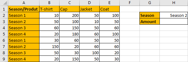
In above screenshot, we can see there is a table record the sales for T-shirts and some other products. Refer to the leftmost column we can see that the sales period contains two cycles of ‘Season1-Season4’. If we want to sum the sales for a specific season, for example season2 in our example, we need to find out all amounts from range B2:E9 belong to season2.

In this case, as we want to sum the sales for season2, so the criterion is season2, and criteria range is A2:A9. We have only one criteria range. As we have four product columns, so in this case we meet the scenario “one criterion with multiple sum columns”.

To sum multiple columns with only one condition, we can apply SUMPRODUCT function.

FORMULA – APPLY SUMPRODUCT FUNCTION

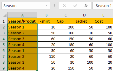
Step 1: Select A2:A9, in Name Box field define it with name “Season”, then when applying a formula, we can directly enter “Season” to represent range “A2:A9”.

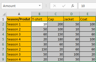
Step 2: Select B2:E9, in Name Box field define it with name “Amount”, then when applying a formula, we can directly enter “Amount” to represent range “B2:E9”.

Step 3: In H3, enter the formula =SUMPRODUCT((Season=H2)*Amount). You can see that we apply a multiplication among SUMPRODUCT.

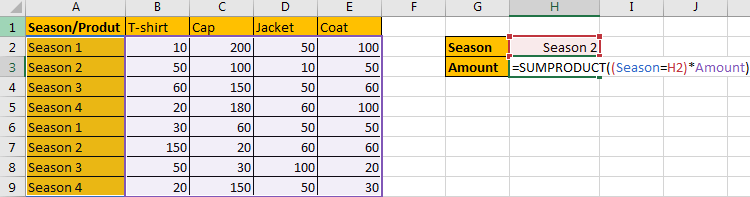
Step 4: Press Enter after typing the formula.

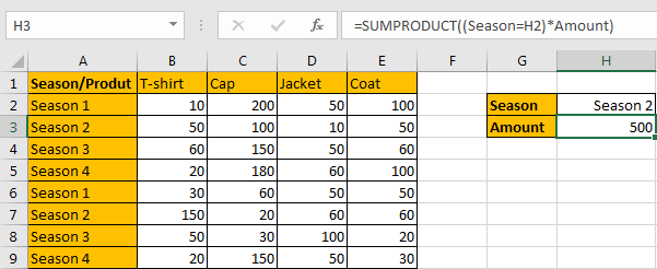
500 is returned by the formula. It is equivalent to “50+100+10+50” in row3 plus “150+20+60+60” in row7. The formula works correctly.

FUNCTION INTRODUCTION

SUMPRODUCT function can be seen as SUM+PRODUCT.

For SUMPRODUCT function, the syntax is:

=SUMPRODUCT(array1,array2,array3, ...)

For example, enter =SUMPRODUCT({1,2},{2,3}) in any cell, the we can get value 8, it equals to 1*2+2*3=8. You can also enter =SUMPRODUCT({1,2}*{2,3}), you can get the same result. The argument array can be a real array {1,2,3} for example or a range reference like A2:A7.

If there is only array in the formula, SUMPRODUCT will sum the numbers in the array.

SUMPRODUCT function allows entering texts, logical operators and expressions like (season=season2), texts should be enclosed into ().

ARGUMENTS EXPLAINATION

In this formula =SUMPRODUCT((Season=H2)*Amount), we only applied SUMPRODUCT one function. And among SUMPRODUCT there is only one multiplication, it is (Season=H2)*Amount, so we have only one argument array1 here. We need to sum the products of this operation.

HOW THIS FORMULA WORKS

For formula =SUMPRODUCT((Season=H2)*Amount, let’s split the formula to several parts and see how to get final result 500 by steps.

For logical operation, we start calculating from the inner part. In the formula bar, select “Amount” in the formula, and press F9 to expand values from “Amount” range reference in an array.

Select (Season=H2) in the formula bar, press F9, then we can get a new array consistent of True and False. In the formula, “Season” represents range A2:A9, if value from this range is equal to “Season 2”, then operation returns True, otherwise it returns False, the result is saved in an array.

In calculation, True is coerced to 1, False is coerced to 0 in calculation. So {FALSE;TRUE;FALSE;FALSE;FALSE;TRUE;FALSE;FALSE} is convert to {0;1;0;0;0;1;0;0}.

So formula is equivalent to

=SUMPRODUCT({0;1;0;0;0;1;0;0}*{10,200,50,100;50,100,10,50;60,150,50,60;20,180,60,100;30,60,50,50;150,20,60,60;50,30,100,20;20,150,50,30})

Select

 {FALSE;TRUE;FALSE;FALSE;FALSE;TRUE;FALSE;FALSE}*{10,200,50,100;50,100,10,50;60,150,50,60;20,180,60,100;30,60,50,50;150,20,60,60;50,30,100,20;20,150,50,30}

in the formula, press F9. We get

 =SUMPRODUCT({0,0,0,0;50,100,10,50;0,0,0,0;0,0,0,0;0,0,0,0;150,20,60,60;0,0,0,0;0,0,0,0})

see screenshot below.

Now values in SUMPRODUCT argument array1 are clear. SUMPRODUCT function will sum these numbers. Select

=SUMPRODUCT({0,0,0,0;50,100,10,50;0,0,0,0;0,0,0,0;0,0,0,0;150,20,60,60;0,0,0,0;0,0,0,0})

in the formula bar, press F9, 500 is displayed in formula bar.

COMMENTS

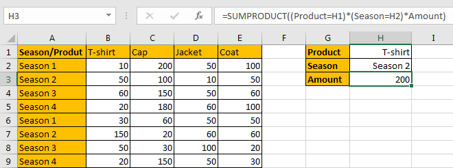
1. If we have two criteria in this case, for example “Product=T-shirt” and “Season=Season 2”, we can still use this formula, just add a new criterion “Product=T-shirt”.

In H3 update the formula =SUMPRODUCT((Product=H1)*(Season=H2)*Amount). Then we can get 200, it is equal to B3+B7=50+150=200.

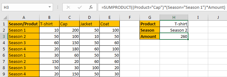
2. If there is no cell to show the criteria like H2=Season 2, we can just enter product or season into the formula. Please make sure that text should be enclosed into double “ ”.

For example, ignore the criteria, just enter =SUMPRODUCT((Product=”Cap”)*(Season=”Season 1″)*Amount) into H3, then we can get total amount for cap in season1.

SUMMARY

1. SUMPRODUCT function can handle multiple arrays, and it sum up the products.

2. SUMPRODUCT function allows user defined range, wildcards, logical operators, expressions.

Related Functions

---

• Excel SUMPRODUCT function
  The Excel SUMPRODUCT function multiplies corresponding components in the given one or more arrays or ranges, and returns the sum of those products. The syntax of the SUMPRODUCT function is as below:= SUMPRODUCT (array1,[array2],…)…