In daily work, if we want to sum numbers from a range, and only sum the numbers which being equal to X or Y in the range, we can create a formula with Excel build-in functions to get the result. In fact, there are many functions can be applied to help us figure out the problem. In this article, we will show you three different ways to resolve this problem by using SUMIFS/SUMIF/SUMPRODUCT functions. We will introduce you the syntax, arguments and basic usage of these functions, and let you know the working process of different formulas.
Table of Contents
EXAMPLE
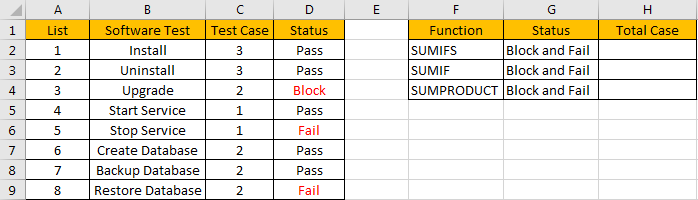
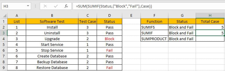
Refer to the left-hand side table, we can see some tasks in software test progress are listed, for each task, there are several related test cases, for example, for task “Install”, there are 3 test cases assigned to it. In “Status” column, there are three status “Pass”, “Fail” and “Block”. For the tasks which status is “Fail” or “Block”, we need to re-test the related test cases, so we need to know how many test cases we need to select and execute in next regression test. Now, we need to calculate the re-run test case number. There are many ways to sum numbers based on specific criteria, for this instance, we will show you how to sum numbers by formula with different functions SUMIF/SUMIFS/SUMPRODUCT. We will enter different formulas into H2, H3, H4 of “Total case” column accordingly in the right-hand side table.
Before designing a formula, we can name range references.
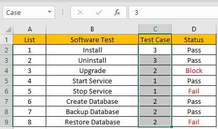
Select range C2:C9, in name box enter ‘Case’, then press Enter.
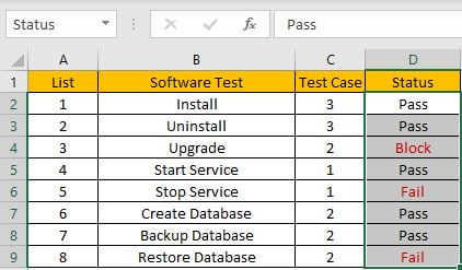
Select range D2:D9, in name box enter ‘Status’, then press Enter.
CREATE A FORMULA with SUM & SUMIFS FUNCTIONS
1.STEPS
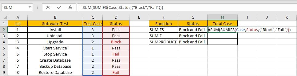
Step 1: In H2, enter the =SUM(SUMIFS(Case,Status,{“Block”,”Fail”})).
=SUMPRODUCT(C2:C9*(D2:D9={"Block","Fail"}))
Step 2: Press Enter after typing the formula.
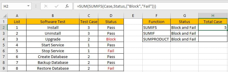
We can see in column D, cell D3, D5 and D8 meet our criteria, so we just need to calculate case numbers from C3, C5 and C8, so the total case number is 2+1+2=5. The formula works correctly.
2.FUNCTION INTRODUCTION
SUM function can add numbers together. It adds all supplied values from a range or a formula.
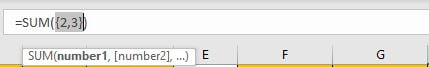
Syntax:
=SUM (number1, [number2], [number3], ...)
SUMIFS function can be seen as SUM+IFS, it can handle multiple ‘criteria range’ and ‘criteria’ combinations.
Syntax:
=SUMIFS(sum_range, criteria_range1, criteria1, [criteria_range2, criteria2], ...)
For both SUM and SUMIFS function, they support wildcards like asterisk ‘*’ and question mark ‘?’, also support logical operators like ‘>’,’<’. If wildcards or logical operators are required, they should be enclosed into double quotes (““).
3.ALL ARGUMENTS
In this case, SUMIFS is included in SUM formula, it is the only argument of SUM function, its returned values should be accumulated by SUM function.
SUMIFS – SUM RANGE
In our instance, range reference ‘Case’ is the ‘sum range’. Test case numbers are listed in this field.
In the formula bar, select ‘Case’, press F9, values in this range are expanded in an array.

SUMIFS – CRITERIA RANGE 1
Range reference ‘Status’ is the criteria range. In this instance we have only one criteria range. We have only three status “Pass”, “Fail” and “Block”.
In the formula bar, select “Status”, pree F9, values in this range are expanded in an array.

SUMIFS – CRITERIA 1
As we want to calculate total test case number for tasks which “status=fail” or “status=block”, so if one condition is matched, test case number will be recorded and accumulated. So, we will supply two criteria “Fail” and “Block” in this case, they are expanded saved in one array, a comma is added between them to split the two criteria. As SUMIFS function supports texts and wildcards, but they should be enclosed into double quotes “”, so for criteria 1, we enter {“Fail”,”Block”}.

Actually, the two criteria can be split to two “criteria1” in two different SUMIFS formulas, for example, if we enter =SUM(SUMIFS(Case,Status,”Fail”),SUMIFS(Case,Status,”Block”)) in H2, we can get the same result.
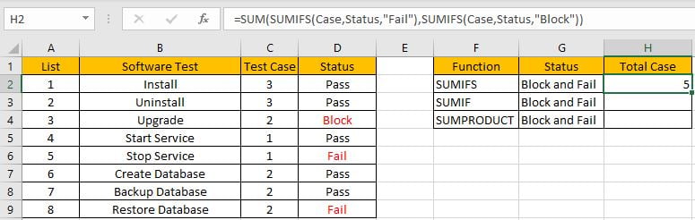
This formula is clear but looks a little bit complex, so we use an array constant with two elements to shorten the formula.
4.HOW THE FORMULA WORKS
After explaining each argument in the formula, now we will show you how the formula works with these arguments.
After expanding values in each range reference, in the formula bar, the formula is displayed as:
=SUM(SUMIFS({3;3;2;1;1;2;2;2},{"Pass";"Pass";"Block";"Pass";"Fail";"Pass";"Pass";"Fail"},{"Block","Fail"}))
If value from the criteria range can match either criteria, “True” will be recorded in this position, otherwise, “False” will be saved instead.
{“Pass”;”Pass”;”Block”;”Pass”;”Fail”;”Pass”;”Pass”;”Fail”} – Criteria Range
{“Block”,”Fail”} – Criteria Collection
So, after comparing, we can get two new arrays based on different criteria:
{False;False;True;False;False;False;False;False} – for criteria “Block”
{False;False;False;False;True;False;False;True} – for criteria “Fail”
For the following logical operation, “True” is coerced to “1” and “False” is coerced to “0”. So above arrays are converted to two arrays only contain numbers “1” and “0”.
{0;0;1;0;0;0;0;0} – for criteria “Block”
{0;0;0;0;1;0;0;1} – for criteria “Fail”
Now, we have below two pairs of arrays:
{3;3;2;1;1;2;2;2} – sum_range
{0;0;1;0;0;0;0;0} – for criteria “Block”
{3;3;2;1;1;2;2;2} – sum_range
{0;0;0;0;1;0;0;1} – for criteria “Fail”
In the two groups, for the elements in the same position, multiply the two elements. Then we can get two new arrays.
{0;0;2;0;0;0;0;0} – for criteria “Block”
{0;0;0;0;1;0;0;2} – for criteria “Fail”
Add all products in above two arrays separately, we get 2 and 3. Actually, if ignore above analysis, directly select SUMIFS part and press F9, a simple array {2,3} is returned.
Now, the SUM function will add the two numbers together, then we get 5 as last.
CREATE A FORMULA with SUM & SUMIF FUNCTIONS
SUMIF function is similar with SUMIFS, they have the same arguments, the difference is it can only handle one criteria range with one criterion, and sum range is listed in the end.
Syntax: =SUMIF(criteria_range, criteria, sum_range)
In this case, all arguments are the same for SUMIF and SUMIFS, as SUMIF only supports one group of criteria range and criteria, so we need to create two SUMIF formulas, and use SUM function to sum two returned values.
In H3, enter the formula =SUM(SUMIF(Status,{“Block”,”Fail”},Case)).
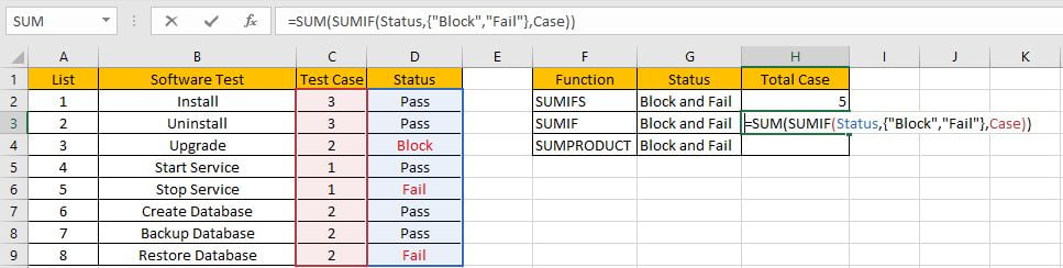
Press Enter to get result. We can see we get the same result.
CREATE A FORMULA with SUMPRODUCT FUNCTION
Different with SUMIFS or SUMIF function, SUMPRODUCT function can directly return proper result and ignore SUM function.
1.STEPS
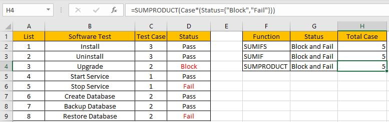
Step 1: In H4, enter the =SUMPRODUCT(Case*(Status={“Block”,”Fail”})).
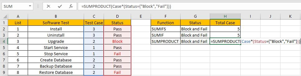
Step 2: Press Enter after typing the formula.
2.FUNCTION INTRODUCTION
SUMPRODUCT function can be seen as SUM+PRODUCT.
Syntax:
=SUMPRODUCT(array1, [array2], [array3], ...)
3.ALL ARGUMENTS
SUMPRODUCT – ARRAY1
In this case, we have only one array, it is a formula “Case*(Status={“Block”,”Fail”})”.
In the formula bar, select “Status”, pree F9, values in this range are expanded in an array.

Compare each status from range ‘Status’ with the criteria, as there are eight elements in criteria range, and two elements in criteria, so after comparing, system will return a two-dimension array (2*8) in the formula bar.
Just select ({“Pass”;”Pass”;”Block”;”Pass”;”Fail”;”Pass”;”Pass”;”Fail”}={“Block”,”Fail”}), then press F9. Verify that comparative result is displayed.

Select “Case”, then press F9, all values from range “Case” are expanded.

4.HOW THE FORMULA WORKS
After expanding values in each range reference, in the formula bar, the formula is displayed as:
=SUMPRODUCT({3;3;2;1;1;2;2;2}*{FALSE,FALSE;FALSE,FALSE;TRUE,FALSE;FALSE,FALSE;FALSE,TRUE;FALSE,FALSE;FALSE,FALSE;FALSE,TRUE})
Notes: For the following logical operation, “True” is coerced to “1” and “False” is coerced to “0”. The formula is updated to =SUMPRODUCT({3;3;2;1;1;2;2;2}*{0,0;0,0;1,0;0,0;0,1;0,0;0,0;0,1}) in calculation progress.
In the formula bar, select {3;3;2;1;1;2;2;2}*{FALSE,FALSE;FALSE,FALSE;TRUE,FALSE;FALSE,FALSE;FALSE,TRUE;FALSE,FALSE;FALSE,FALSE;FALSE,TRUE} and press F9. We can see that one new array consists of products of previous two arrays are listed.
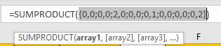
Select =SUMPRODUCT({0,0;0,0;2,0;0,0;0,1;0,0;0,0;0,2}), press F9 to do the last step – SUMPRODUCT function will add products in the array together. As 2+1+2=5, so we get 5 by this formula.
![]()
SUMMARY
1. SUMIFS function can handle multiple groups of criteria ranges and criteria. Sum range is the first argument among all arguments.
2. SUMIF function can handle only one pair of criteria range and criteria. Sum range is the last argument among all arguments.
3. SUMPRODUCT function can return the sum of products.
4. They all support wildcards, logical operators.
Related Functions
- Excel SUMPRODUCT function
The Excel SUMPRODUCT function multiplies corresponding components in the given one or more arrays or ranges, and returns the sum of those products.The syntax of the SUMPRODUCT function is as below:= SUMPRODUCT (array1,[array2],…)… - Excel SUMIFS Function
The Excel SUMIFS function sum the numbers in the range of cells that meet a single or multiple criteria that you specify. The syntax of the SUMIFS function is as below:=SUMIFS (sum_range, criteria_range1, criteria1, [criteria_range2, criteria2], …)… - Excel SUMIF Function
The Excel SUMIF function sum the numbers in the range of cells that meet a single criteria that you specify. The syntax of the SUMIF function is as below:=SUMIF (range, criteria, [sum_range])…