In previous articles, we have introduced you some ways to sum data by group, month, weekday, week number etc. Actually, in our work life, we may meet some situations a bit more complex than above-mentioned cases. Depends on different situations, we may sum data by applying different formulas within different excel functions.
Table of Contents
Sum Data Based on Criteria Adjacent Columns
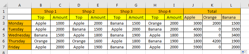
Suppose we have four fruit shops, and only supply three different fruits for example apple, banana, orange. On different weekdays, each shop has its own high sales fruit. See example in below screenshot.
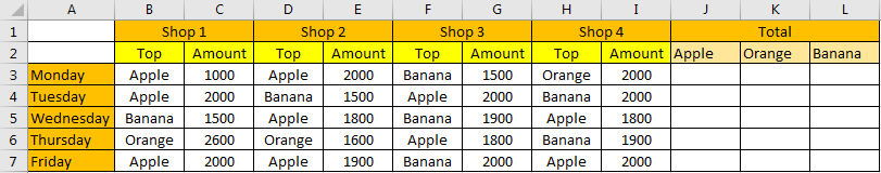
Here’s the question, among the top sales fruits, if we want to know which fruit has the highest sales on each weekday, how can we do?
Actually, this instance can be seen that to sum data based on values in different columns. Refer to above screenshot, to sum amount for Apple on Monday, we need to pick up Apple in B,D,F,H these four columns, and then sum amount from their adjacent columns C,E,G,I. In this instance, we can apply SUMPRODUCT function to solve our problem.
This article will show you ‘sum data by columns’ by only applying excel SUMPRODUCT function. We will use above instance to show you how to sum data based on criteria adjacent columns. We will introduce you the usage of SUMPRODUCT function with simple descriptions, screenshots and explanations. I’m sure that you can learn sum data based on columns by formula clearly by yourself after reading this article, you can work well with this function in your daily work in the future.
FORMULA:
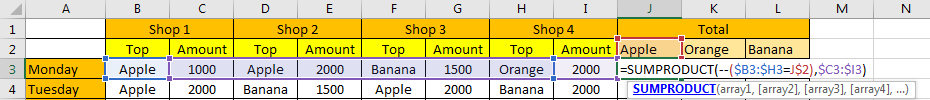
In cell J3 enter the formula =SUMPRODUCT(–($B3:$H3=J$2),$C3:$I3).
After clicking Enter to applying the formula, you can see that 3000 is returned in J3.
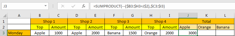
Refer to above screenshot, we can see that Apple appears in B3 and D3, so we extract data from adjacent columns C3 and E3, in C3 the value is 1000, in E3 the value is 2000, so the returned value 3000 is correct, that confirms the formula works correctly.
HOW THIS FORMULA WORKS:
This formula is based on SUMPRODUCT function. SUMPRODUCT function syntax has the following arguments:
=SUMPRODUCT(array1, [array2], [array3], …)
In this instance, in the formula =SUMPRODUCT(–($B3:$H3=J$2),$C3:$I3). There are two arrays, the first array is –($B3:$H3=J$2), the second array is $C3:$I3. We will explain the formula work process by analysis each array one by one.
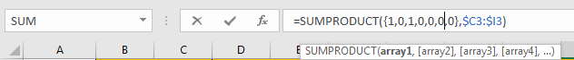
For –($B3:$H3=J$2), B3:H3 contains all top sales fruit cells on Monday (and three amount cells); we add $ before column B and H to make columns are not changed when applying the formula for other criteria for example K2 (Orange); after adding $ before each column number, the two columns are locked and will not automatically updated in the formula. Just select ($B3:$H3=J$2) in the formula, and press F9, then actual values in the instance are displayed in the formula bar. See screenshot below.
![]()
In this argument, we compare each value in B3:H3 with J2 value. For example, the first value is ‘Apple’, it equals to the criteria ‘Apple’, so we get TRUE here; but for the second value in the array ‘1000’, it doesn’t match to ‘Apple’, so we get FALSE here. After comparing all values in the array with criteria, we get the returned value array {TRUE,FALSE,TRUE,FALSE,FALSE,FALSE,FALSE}. Only texts TRUE and FALSE display in the array.

As function cannot work with text TRUE or FALSE, so they are forced to be converted to numbers. Convert FALSE to 0 and TRUE to 1 for the following process. So, the array is updated to {1;0;1;0;0;0;0}.
For the second array $C3:$I3, C3:I3 contains all amount values on Monday (and three fruit cells). We also add $ before column to make columns are locked when applying the formula for other criteria. Select $C3:$I3 in the formula, and press F9, then actual values in this instance are displayed in the formula bar.

So, SUMPRODUCT(–($B3:$H3=J$2),$C3:$I3) can be seen as values in one array is multiplied by the values in another array:
{1;0;1;0;0;0;0}*{1000,”Apple”,2000,”Banana”,1500,”Orange”,2000}={1000;0;2000;0;0;0;0}. Then sum the values in the array, the final result is 3000. In this step, SUMPRODUCT can ignore the error that caused by values multiply texts in the array actually, so don’t worry about texts exist in array.
RESULT:
Let’s see if this formula works correctly for other criteria.
Select J3, hold and drag the handle to cover other blank cells in the table, then release. Verify that formula is copied and applied in ‘Total’ area properly.
Select L4 to check if the formula is copied properly.
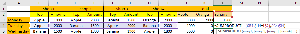
Verify that array and criteria are selected properly, the formula works well.
NOTES:
1. If you are confused about the parameters in the formula, you can just remember commonly used formula for SUMPRODUCT:
=SUMPRODUCT(–(criteria range=criteria), sum range)
In this formula, just select a criteria range that contains your criteria, then select your criteria, and at last confirm your sum range.
2. We can also apply SUMIFS function to calculate total amount for each fruit instead of SUMPRODUCT function in another way.
Enter the formula =SUMIFS($C3:$I3,$B3:$H3,J$2) into J2.
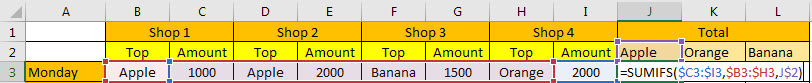
After pressing Enter, 3000 is displayed properly. See screenshot below.
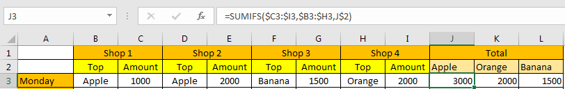
Even though texts exist in sum range, they can be ignored and only proper values are involved in the formula processing. So, in J2, the formula can been seen as =SUMIFS({1000,”Apple”,2000,”Banana”,1500,”Orange”,2000},{“Apple”,1000,”Apple”,2000,”Banana”,1500,”Orange”},”Apple”). In previous articles, we have told you the usage of SUMIFS function and how to use SUMIFS function to sum data, you can search SUMIFS and check related articles on our website freely.
![]()
Related Functions
- Excel SUMPRODUCT function
The Excel SUMPRODUCT function multiplies corresponding components in the given one or more arrays or ranges, and returns the sum of those products. The syntax of the SUMPRODUCT function is as below:= SUMPRODUCT (array1,[array2],…)… - Excel SUMIFS Function
The Excel SUMIFS function sum the numbers in the range of cells that meet a single or multiple criteria that you specify. The syntax of the SUMIFS function is as below:=SUMIFS (sum_range, criteria_range1, criteria1, [criteria_range2, criteria2], …)…