Sometimes we may meet the case that to sum numbers based on two or more specific criteria. In this article, we will show you the method to resolve this problem by formulas with the help of Excel SUMPRODUCT function. SUMPRODUCT can filter data based on the supplied specific criteria and then sum up the filtered numbers properly.
Through a simple instance below, we will introduce you the syntax, argument and the usage of SUMPRODUCT function. We will let you know how the formula works step by step to reach your goal clearly. After reading the article, you may have a simple understanding of SUMPRODUCT function.
Table of Contents
EXAMPLE
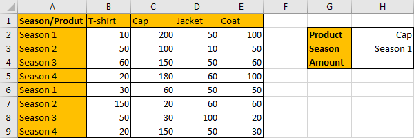
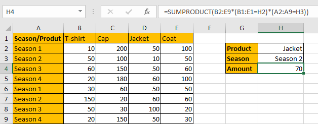
Refer to the left-hand table, we can see it is a 2D table. It contains “Product” and “Season” two criteria, and range B2:E9 shows the amount for different products in different cycle of seasons. In the right-hand table, it is a simple summary table, it calculates the total amount based on supplied product and season. Above all, we can know that there are two criteria “Product” and “Season”, our expectation is counting the total amount of product “Cap” in specific period “Season 1”. In this case, actually user can change product and season in H column, the two values are dynamic values. But when applying the formula, we just use cell reference H2 and H3 to represent the value, so, if H2 or H3 value is changed, the returned value is also changed accordingly.
As we want to sum numbers from range B2:E9 based on the criteria “Product=Cap & Season=Season 1”, we need to find out all numbers that can meet our requirement, and then sum up. To resolve this issue by formula, we can apply Excel SUMPRODUCT function.
FORMULA – APPLY SUMPRODUCT FUNCTION
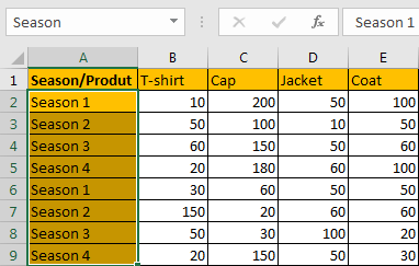
Step 1: Select A2:A9, then in Name Box define a name for this column, just use the column header ‘Season’.
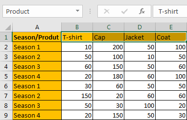
Step 2: Select B1:E1, in Name Box define a name for this row, for example ‘Product’.
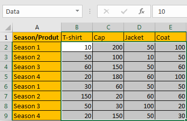
Step 3: Select B2:E9, in Name Box define a name for this range, for example ‘Data’.
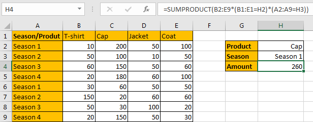
Note: Above three steps are not required, they are optional, you can directly use cell or range reference like A2:A9, B1:E1 in your formula, but for understanding well, we name ranges in advance.
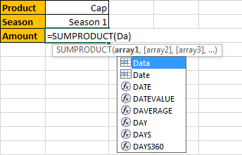
Step 4: In H4, enter the formula =SUMPRODUCT(Data*(Product=H2)*(Season=H3)).
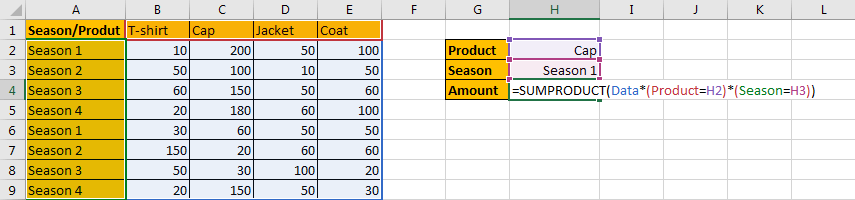
Note: In above steps we already name ranges “Season”,“Product” and “Data”, so when entering the range information into the formula, just after typing “Da…”, our named range “Data” is loaded, just select it from dropdown list.
Step 5: Press Enter after typing the formula.
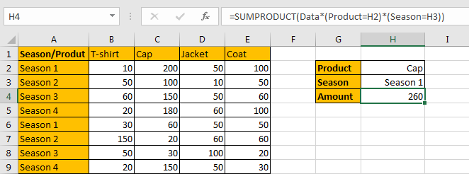
We can see that only cell C2 and C6 can meet the two conditions (Product=Cap) and (Season=Season 1), so, values from C2 (200) and C6 (60) are summed, the total amount is 200+60=260. The formula works correctly.
SUMPRODUCT FUNCTION INTRODUCTION
SUMPRODUCT function can be seen as SUM+PRODUCT.
For SUMPRODUCT function, the syntax is:
=SUMPRODUCT(array1,array2,array3, …)
The values in arrays are multiplied correspondingly, then sum up the products. For example, enter =SUMPRODUCT({1,2,3},{2,3,4}) in any cell, the we can get value 20, it equals to 1*2+2*3+3*4=20.
SUMPRODUCT function allows entering texts, logical operators and expressions like (product=cap), texts should be enclosed into ().
SUMPRODUCT ARGUMENTS EXPLAINATION
SUMPRODUCT – RANGE 1 – Sum Range
Refer to the left table, we know that the main range is “Data”, it records the amounts for each product in different seasons. In this range, we filter data by two criteria, and then sum up the filtered data. In the formula bar, select “Data”, press F9, we can see that values from range B2:E9 are listed properly.

SUMPRODUCT – RANGE 1 – Criteria 1
In the right table, we know that there are two criteria (Product=Cap) and (Season=Season 1). As “Cap” is saved in H2, we directly use cell reference H2 into the formula to represent “Cap”, So we enter (Product=H2) as one criterion. We can also change cap to other product in H2, the returned value will be updated based on the changing.
In the formula bar, select Product, press F9, and then select H2, press F9. All products are listed in an array. Then we get a logical expression ({“T-shirt”,”Cap”,”Jacket”,”Coat”}=”Cap”).

SUMPRODUCT – RANGE 1 – Criteria 2
(Season=Season 1) is another criterion, “Season 1” is saved in H3. Select “Season” and “H3” in the formula bar, press F9. Then we get a logical expression {“Season 1″;”Season 2″;”Season 3″;”Season 4″;”Season 1″;”Season 2″;”Season 3″;”Season 4″}=”Season 1”).

SUMPRODUCT WORKFLOW
After explaining argument in the formula, now we will show you how the formula works with the help of these arrays and expressions.
=SUMPRODUCT({10,200,50,100;50,100,10,50;60,150,50,60;20,180,60,100;30,60,50,50;150,20,60,60;50,30,100,20;20,150,50,30}*({"T-shirt","Cap","Jacket","Coat"}="Cap")*({"Season 1";"Season 2";"Season 3";"Season 4";"Season 1";"Season 2";"Season 3";"Season 4"}="Season 1")).
We have two logical expressions
{“T-shirt”,”Cap”,”Jacket”,”Coat”}=”Cap”
{“Season 1″;”Season 2″;”Season 3″;”Season 4″;”Season 1″;”Season 2″;”Season 3″;”Season 4″}=”Season 1”
Select the two expressions in the formula bar, press F9, we can get two arrays combined with “True” and “False”, they are the results of the two expressions.
=SUMPRODUCT({10,200,50,100;50,100,10,50;60,150,50,60;20,180,60,100;30,60,50,50;150,20,60,60;50,30,100,20;20,150,50,30}*{FALSE,TRUE,FALSE,FALSE}*{TRUE;FALSE;FALSE;FALSE;TRUE;FALSE;FALSE;FALSE})

Convert ‘True’ to ‘1’ and ‘False’ to ‘0’ to make the two arrays can be taken into calculation in next step. (Actually, the two arrays are multiplied in this step if we select both of them and press F9. So, we get only one array that contains 1 and 0.)

Now, we have below two arrays:
{10,200,50,100;50,100,10,50;60,150,50,60;20,180,60,100;30,60,50,50;150,20,60,60;50,30,100,20;20,150,50,30}

{0,1,0,0;0,0,0,0;0,0,0,0;0,0,0,0;0,1,0,0;0,0,0,0;0,0,0,0;0,0,0,0})
Multiply the two arrays. Select the two arrays, press F9.
![]()
Then sum up all the values in this array. We get 200+60=260 at last.
NOTE
- If we didn’t name ranges, we can select range in formula directly.
2. f values are changed in H2 and H3, the returned value is also updated accordingly.
SUMMARY
1. SUMPRODUCT function can handle multiple arrays, and it sum up the products of these arrays.
2.SUMPRODUCT function allows user defined range, wildcards, logical operators, expressions.
Related Functions
- Excel SUMPRODUCT function
The Excel SUMPRODUCT function multiplies corresponding components in the given one or more arrays or ranges, and returns the sum of those products.The syntax of the SUMPRODUCT function is as below:= SUMPRODUCT (array1,[array2],…)…