This post will guide you how to reverse the order of a chart Axis in your current worksheet in Excel 2013/2016.

Assuming that you have created a column chart based on your data in your worksheet, and you may want to reverse the Axis order in this chart. How to do it. And his post will show you one method to accomplish the result of reversing Axis order in your chart.

1. Reverse Axis Order in a Chart

To reverse Axis Order in a chart, you need to create a chart based on your original data firstly, and then do the following steps:

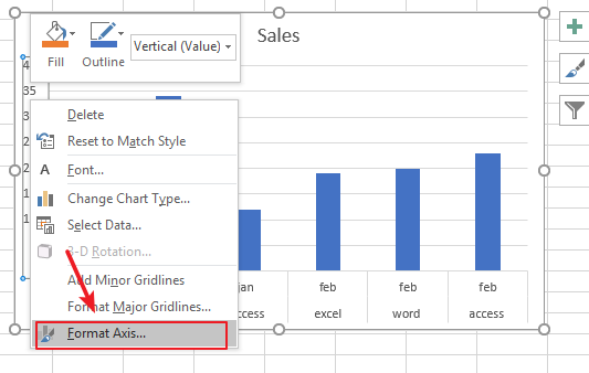
Step1:  right click on one Axis that you want to reverse, such as: X Axis or Y Axis, and then select Format Axis option from the drop down menu list. And the Format Axis pane would be displayed in the left of Excel window.

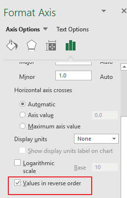
Step2: check values in reverse order or Categories in reverse order option under the Axis Options section in the Format Axis pane.

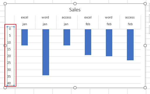
Step3: close the Format Axis pane, and you would see that the selected Axis is reversed.

2. Video: Reverse Axis Order in a Chart

This Excel video tutorial, where we’ll dive into the process of reversing axis order in your Excel charts for a clearer visual representation of your data.