Sometimes we may want to only sum the visible cells in a filtered list or a table. We may notice that if we use SUM function directly with selecting the visible reference in the filtered list, all data in the list (also contains the hidden rows) is included into calculation.
Table of Contents
1. Only Sum Visible Cells/Rows in a Filtered List using Formula
Above all, we need to find a proper function can only sum visible cells in a filtered list and ignore the filtered-out data. Actually, excel built-in SUBTOTAL function can perform calculating like sum data, count, average for both visible & invisible cells or only visible cells properly. As we only want to show you the formula to perform sum visible cells in filter list, so in this article we will only introduce you the basic usage of SUBTOTAL function on sum data. After reading this article, I think you must have a well understanding of SUBTOTAL function, it is flexible for you to use it in your daily work.
EXAMPLE:
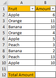
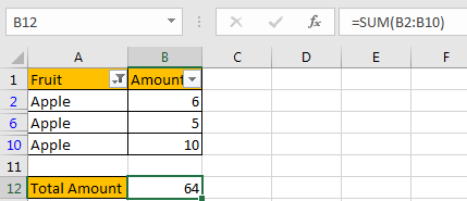
If we want to sum total amount for the filtered fruit, can we use SUM function here directly?
Enter =SUM(B2:B10) in B12. See screenshot below, we get 64 here, the returned value is incorrect obviously. It equals to the total amount of the whole list B2:B10, the hidden rows are also taken into calculation.
FORMULA:
Let’s apply SUBTOTAL function in this case to try to calculate total amount for ‘Apple’ again.
Step 1: Enter
=SUBTOTAL(9,B2:B10)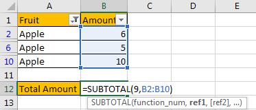
Step 2: Press Enter to load return value.
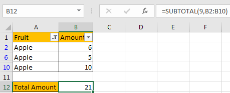
We can see that this time correct amount 21 is displayed in B12.
HOW THIS FORMULA WORKS:
This formula only contains only one function: SUBTOTAL function.
Syntax:
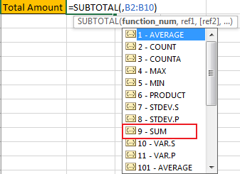
=SUBTOTAL (function_num, ref1, [ref2], ...)It has several arguments like function_num, ref1, ref2. For function_num, it is a number, it shows the function used by SUBTOTAL, by providing different numbers, SUBTOTAL function can perform different calculation. As we mentioned above, SUBTOTAL function can perform most basic calculations like SUM, COUNT, AVERAGE, etc., so we need to know some useful function numbers before explaining SUBTOTAL function.
Please see below screenshots, they show the correspondence between number and function.
Function number from 1 – 101.
Function number from 101 – 111.
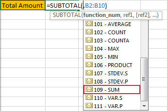
Refer to above function number list, we can see that SUM function has two function numbers, 9-SUM and 109-SUM. Actually, if we enter 9, SUBTOTAL function will only sum visible data and ignore the filtered-out data; and if we enter 109, SUBTOTAL function will only sum visible data and ignore the manually hidden data. See, the difference is:
9: ignore data which is hidden by filter list;
109: ignore data which is hidden manually.
In this instance, in the formula =SUBTOTAL(9,B2:B10). There are two arguments. For the first argument function_num, as data is hidden by filter list, so we enter 9 here; for the second argument, reference, we can enter the whole list B2:B10, or you can also hold your mouse and select the visible cells directly.
RESULT:
We already get proper amount for ‘Apple’, this time let’s pick Banana to check if our formula works properly after changing the filter criteria.
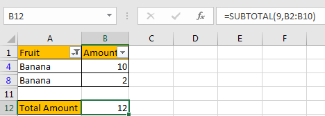
It works properly. SUBTOTAL function can work well on ‘sum visible cells’.
NOTES:
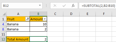
- If we change function_num from 9 to others, the SUBTOTAL function will change calculation accordingly based on the function number. For example, change 9 to 2 in this case (2 – COUNT).
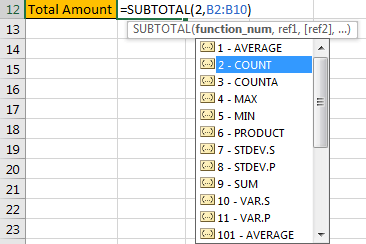
We will get 2 by applying the formula.
- SUBTOTAL function can ignore all hidden data, so we can also use it to sum visible cells in a range. Just enter the range as the reference, the it will ignore hidden cells in this range.
2. Only Sum Visible Cells/Rows in a Filtered List using VBA Code
Now, let’s delve into the second method, which employs VBA code to achieve the same outcome.
For a more programmatic approach, VBA (Visual Basic for Applications) code provides flexibility in summing visible cells.
Press Alt + F11 to open the VBA editor.
Right-click in the Project Explorer, select Insert, and choose Module to create a new module.
Copy and paste the following VBA code into the module:
Function SumVisibleCells(rng As Range) As Double
    Dim cell As Range
    Dim total As Double

    For Each cell In rng
        If cell.EntireRow.Hidden = False And IsNumeric(cell.Value) Then
            total = total + cell.Value
        End If
    Next cell

    SumVisibleCells = total
End Function
This code defines a custom function SumVisibleCells that sums only visible cells in a given range.
Return to your Excel sheet and use the custom function
Type this formula:
=SumVisibleCells(B2:B10)Adjust the range as needed.
By following these steps, you’ll employ VBA code to sum only visible cells in a filtered list.
3. Video: Only Sum Visible Cells/Rows in a Filtered List
This Excel video tutorial on effectively summing only visible cells or rows in a filtered list. We’ll explore two methods to achieve this task seamlessly: utilizing a formula based on the SUBTOTAL function and employing VBA code.
4. Related Functions
- Excel SUBTOTAL function
The Excel SUBTOTAL function returns the subtotal of the numbers in a list or database. The syntax of the SUBTOTAL function is as below:= SUBTOTAL (function_num, ref1, [ref2])…. - Excel SUM function
The Excel SUM function will adds all numbers in a range of cells and returns the sum of these values. You can add individual values, cell references or ranges in excel.The syntax of the SUM function is as below:= SUM(number1,[number2],…)…