This post will guide you how to highlight the highest value in each row or column in Excel. How do I highlight the lowest value in each row and column with conditional formatting function.
Table of Contents
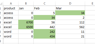
Highlight Highest Value in Each Row
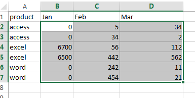
Assuming that you have a list of data in range A1:D7, and you want to highlight all highest values in each row or highlight all lowest values in each row. How to achieve it. You need to use the conditional formatting feature to achieve the result. Just do the following steps:
#1 select the range of cells that you want to highlight the highest values in each row.
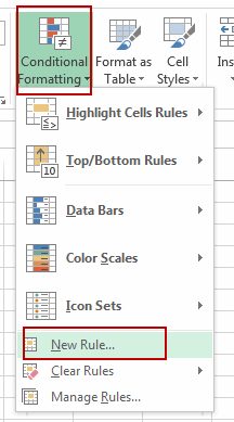
#2 go to HOME tab, click Conditional Formatting command under Styles group. And then select New Rule from the drop down menu list. And the New Formatting Rule dialog will appear.
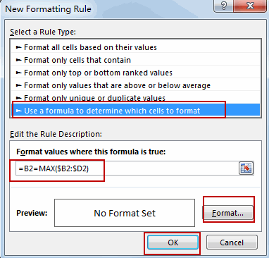
#3 select Use a formula to determine which cells to format in the Select a Rule Type list box, and type the following formula in the Format values where this formula is true text box. And then click Format button.
=B2=MAX($B2:$D2)
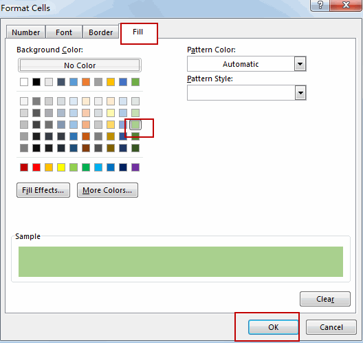
#4 switch to Fill tab, select on background color as you need. Click Ok button.
#5 click Ok button. The highest value in each row has been highlighted.
Highlight Lowest Value in Each Row
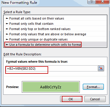
If you want to highlight lowest value in each row in your table, you just need to repeat the above steps, just use the following formula instead of it.
=B2=MIN($B2:$D2)
Highlight Highest Value in Each Column
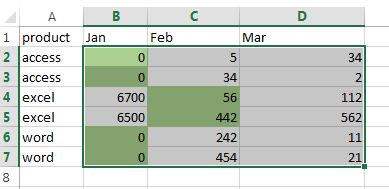
If you want to highlight highest value in one column, you can repeat the above steps, and then use the following formula:
=B2=MAX($B$2:B$7)
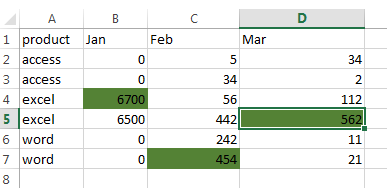
Highlight Lowest Value in Each Column
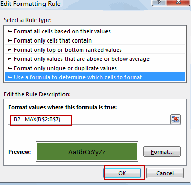
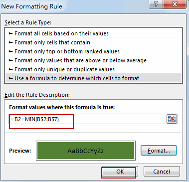
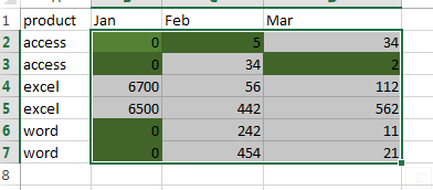
If you want to highlight highest value in one column, you can repeat the above steps, and then use the following formula:
=B2=MIN(B$2:B$7)
Video: Highlight Highest and Lowest Values in each Row or Column
Related Functions
- Excel MIN function
The Excel MIN function returns the smallest numeric value from the numbers that you provided. Or returns the smallest value in the array.The MIN function is a build-in function in Microsoft Excel and it is categorized as a Statistical Function.The syntax of the MIN function is as below:= MIN(num1,[num2,…numn])…. - Excel MAX function
The Excel MAX function returns the largest numeric value from the numbers that you provided. Or returns the largest value in the array.= MAX(num1,[num2,…numn])…
Leave a Reply
You must be logged in to post a comment.