In our daily work, we often find some duplicate values in a certain range. For example, when accounting the profits for different salespersons in a week, they may make the same profit on different days, or they may have the same total profits for the whole week. If we want to highlight all duplicate profits or highlight the entire rows with only the duplicate total profits, how can we do? Actually, we can through conditional formatting function to highlight duplicate values or rows/columns with duplicate values for different situations accordingly. This free tutorial will show you the details to highlight duplicate values for above two cases.
Precondition:
See screenshot below. There are some duplicate values in the table.
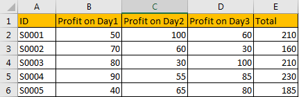
Table of Contents
1. Highlight All Duplicate Values in the Entire Table
If we just want to find all duplicate values without any limit, we can directly highlight them by applying ‘Duplicate Values’ rule in conditional formatting function. See details below.
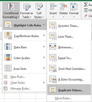
Step 1: Select the entire table. Then click Home in ribbon, click the small triangle on Conditional Formatting icon (in Styles group), then select Highlight Cells Rules->Duplicate Values option.
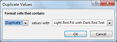
Step 2: Just keep default settings in pops up ‘Duplicate Values’ dialog. You can also change color in ‘values with’, then click OK.
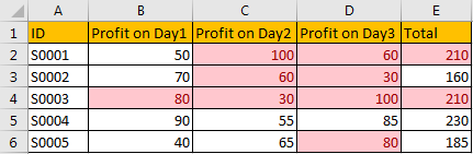
Step 3: Check result below. All duplicate values are highlighted.
2. Highlight the Entire Row or Column with Duplicate Values
In this example, we want to highlight the entire rows if they have the same Total values.
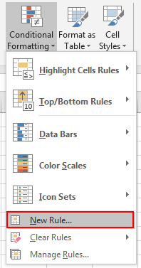
Step 1: Select the entire table, this is important. Click Home in ribbon, then click Conditional Formatting in Styles group, select New Rule in menu.
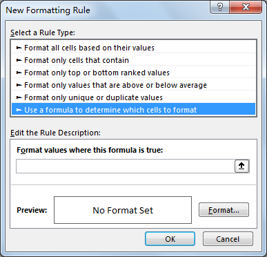
Step 2: On New Formatting Rule dialog, select the last rule type: Use a formula to determine which cells to format.
Step 3: In Edit the Rule Description section, in Format values where this formula is true textbox enter the formula
=COUNTIF($E$2:$E$6,$E2)>1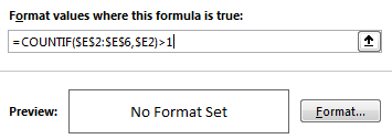
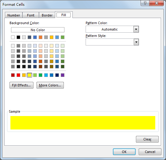
Step 4: Click Format button in Preview section. Verify that Format Cells window is displayed.
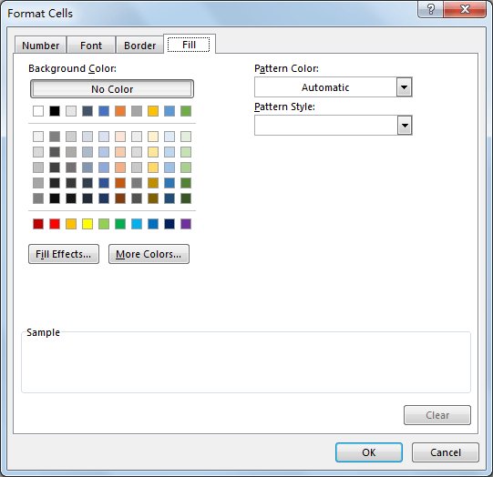
Step 5: Click Fill tab, then select a color as background color. For example, select yellow, then click OK.
Step 6: After above step, we go back to New Formatting Rule window. You can see that in Preview section, cell is filled with yellow. Click OK.

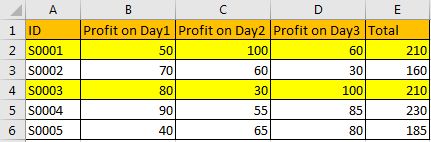
Step 7: Check the result below. You can see that entire rows with duplicate total values are highlighted.
3. Video: Highlight All Duplicate Values
This Excel video tutorial will take you through two effective methods that utilize Excel’s conditional formatting to identify and highlight duplicate values.
4. Related Functions
- Excel COUNTIF function
The Excel COUNTIF function will count the number of cells in a range that meet a given criteria. This function can be used to count the different kinds of cells with number, date, text values, blank, non-blanks, or containing specific characters.etc.= COUNTIF (range, criteria)…