This post will guide you how to transpose horizontal list to vertical list in your current worksheet in Excel. How do I convert horizontal rows to vertical columns with a formula in Excel 2013/2016.

• Convert Horizontal List to Vertical with a Formula
• Convert Horizontal List to Vertical using Paste Special Feature

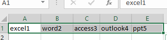
Assuming that you have a list of data (A1:E1) in a Microsoft Excel worksheet, and you want to realize that the data you entered in rows makes better sense in columns or vice versa. You need to transpose your rows and columns from horizontal list to vertical list. This post will show you two methods to change the horizontal row style to vertical style.

Convert Horizontal List to Vertical with a Formula

---

If you want to convert horizontal list to a vertical list, you can create a formula based on the INDEX function in combination with ROWS function. Like this:

=INDEX(A$1:E$1, ROWS(F$1:F1))

Then enter this formula into a blank cell such as: Cell F1, and then press Enter key on your keyboard, and the drag the AutoFill Handle down to other cells, until you get a #REF! error message.

Note: Cell A1:E1 is your horizontal list, and F1 is the first cell that you want to place vertical list. It is also the cell that you want to apply for the formula.

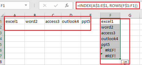
You would see that the horizontal list has been converted to vertical list.

 

Convert Horizontal List to Vertical using Paste Special Feature

---

You can also use Paste Special function to achieve the same result of transposing horizontal row data into vertical column style in Excel. Just do the following steps:

Step1: select cells that you want to convert, such as: A1:E1.

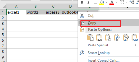
Step2: right click on the selected cells, and select Copy option from the popup context menu.

Step3: select a blank cell that you want to place vertical list, such as: Cell F1. And right click on it , and choose Paste Special from the popup menu list. Then the Paste Special dialog will open.

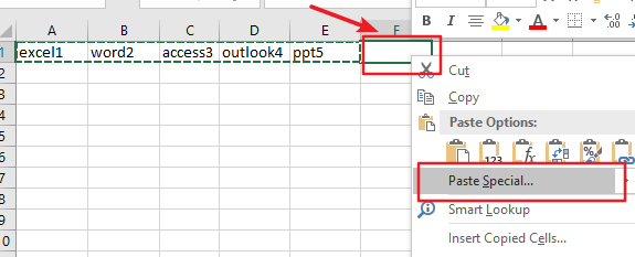
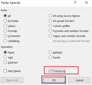
Step4: check the Transpose box in the Paste Special dialog box. Then click Ok button.

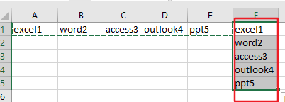
Step5: you would now see your horizontal data be transposed to vertical style.

Related Functions

---

• Excel INDEX function
  The Excel INDEX function returns a value from a table based on the index (row number and column number)The INDEX function is a build-in function in Microsoft Excel and it is categorized as a Lookup and Reference Function.The syntax of the INDEX function is as below:= INDEX (array, row_num,[column_num])…
• Excel ROWS function
  The Excel ROWS function returns the number of rows in a cell reference.The syntax of the ROWS function is as below:= ROWS(array)…