This post will guide you how to convert an Excel Table to a range of data in Excel. How do I convert data in Excel into a Table.

• Convert Data to a Table
• Convert an Excel Table to a Range of Data

Convert Data to a Table

---

If you want to convert a range of data to a table in your current worksheet, just do the following steps:

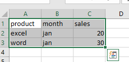
Step1: select the data range that you want to convert, such as: A1:C3

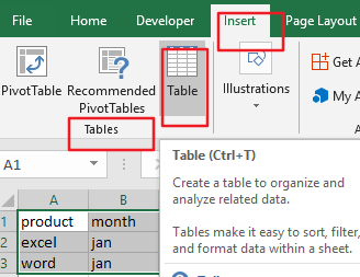
Step2: go to Table tab in the Excel Ribbon, click Table command under Tables group. And the Create Table dialog will open.

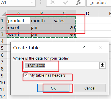
Step3: check My table has headers in the Create Table dialog box, click Ok button.

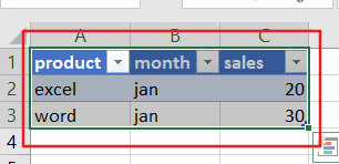
Step4: you would see that your selected data has been converted to a table.

 

Convert an Excel Table to a Range of Data

---

Assuming that you have created an Excel table in your current worksheet, and you want to remove the table style without the functionality. And you want to stop working with your data in a table without losing any table style formatting that you applied, you can convert the table to a regular range of data on the current worksheet, just do the following steps:

Step1: click any cell in the table, and go to Table Tools->Design.

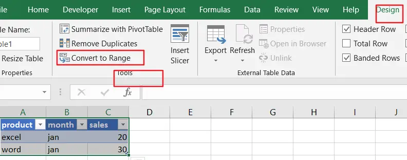
Step2: click Convert to Range command under Tools group. One Warning dialog box will appear.

 

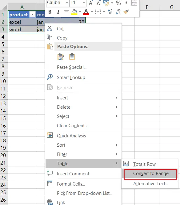
Or you can also right click on the table, and then click Table from the drop down menu list, and then select Convert to Range.

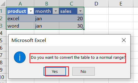
Step3: click Yes button to confirm that you want to convert the table to a normal range.