How to Calculate Average Ignore Non-Numeric Values and Errors

In daily work we often need to calculate the average of some numbers in a range for further analysis. Thus, we need to know some basic functions of calculate average in Excel. From now on, we will introduce you some basic functions like AVERAGE, AVERAGEIF, and show you some common formulas to calculate average value.

In this article, we will let you know how to calculate average by AVERAGE function easily and the way to calculate average based on a given criteria by AVERAGEIF function. We will introduce you the syntax, arguments, and basic usage about the two functions, and let you know the working process of our created formulas.

Table of Contents

1. EXAMPLE
2. CREATE A FORMULA with AVERAGEIF FUNCTION
- a. FUNCTION INTRODUCTION
- b. HOW THE FORMULA WORKS
3. Calculate Average Ignore Non-Numeric Values and Errors with VBA Code
4. Related Functions

1. EXAMPLE

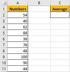
Refer to “Numbers” column, some numbers are listed in range A2:A11. C2 is used for entering a formula which can calculate the average of numbers in range A2:A11. In fact, Excel has amount of built-in functions and they can execute most simple calculations properly, and AVERAGE is one of the most common used functions.

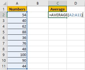
In C2, enter “=AVERAGE(A2:A11)”.

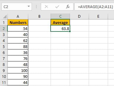
Then press Enter, AVERAGE function returns 63.8.

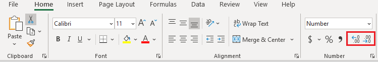
You can adjust decimal places by “Increase Decimal” or “Decrease Decimal” in “Number” section.

But if some errors or blank or non-numeric values exist in the list, how can we only calculate average for numbers ignoring the invalid values? See example below.

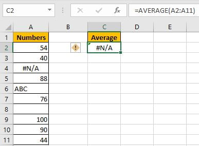
We get an error when calculating average for range A2:A11, the difference is there are some invalid values in the list. To calculate average ignoring the errors, that means we need to calculate average of numbers in a range with one or more criteria, thus, we can apply AVERGAEIF function instead of basic AVERAGE function.

2. CREATE A FORMULA with AVERAGEIF FUNCTION

Step1: In C2, enter the formula =AVERAGEIF(A2:A11,”>0″).

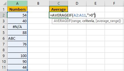
You can also name range “Numbers” for A2:A11, then you can enter =AVERAGEIF(Numbers,”>0″).

Step2: Press Enter after typing the formula.

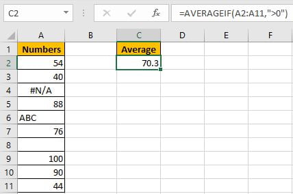
Ignore the improper cells, and only calculate the average of numbers 54, 40, 88, 76, 100, 90 and 44, total 7 numbers. (54+40+88+76+100+90+44)/7=70.3. The formula works correctly.

a. FUNCTION INTRODUCTION

AVERAGEIF function is AVERAGE+IF. It returns the average of some numbers in a range based on given criteria.

Syntax:

=AVERAGEIF(range, criteria, [average_range])

It supports wildcards like asterisk ‘*’ and question mark ‘?’, also supports logical operators like ‘>’,’<’. If wildcards or logical operators are required, they should be enclosed into double quotes (““), in this case we entered “>0” to show the criteria.

AVERAGEIF – RANGE

This example is very simple, we have only one list. A2:A11 is criteria range and average range.

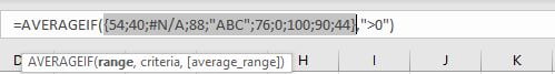
In the formula bar, select “A2:A11”, press F9, values in this range are expanded in an array.

If average range=criteria range, average range can be omitted.

AVERAGEIF – CRITERIA

Obviously, the criteria in our case is “>0”, this condition can filter numbers from criteria range.

b. HOW THE FORMULA WORKS

After expanding values, the formula is displayed as:

=AVERAGEIF({54;40;#N/A;88;"ABC";76;0;100;90;44},">0")

Note: blank cell is recorded as 0 in the array.

Because of criteria “>0”, so invalid cells are ignored. Replace all invalid values with 0. Keep all numbers.

{54;40;#N/A;88;"ABC";76;0;100;90;44} -> {54;40;0;88;0;76;0;100;90;44}

Now this new array only contains numbers. We can calculate the average now.

3. Calculate Average Ignore Non-Numeric Values and Errors with VBA Code

You can also create a User Defined Function to calculate the average of a range of cells, ignoring any non-numeric values or error values, just do the following steps:

Step1: Click on the “Visual Basic” button in the Developer tab to open the Visual Basic Editor.

Step2: In the Visual Basic Editor, click on “Insert” in the menu and select “Module” to create a new module.

Step3: Paste the VBA code provided in the new module.

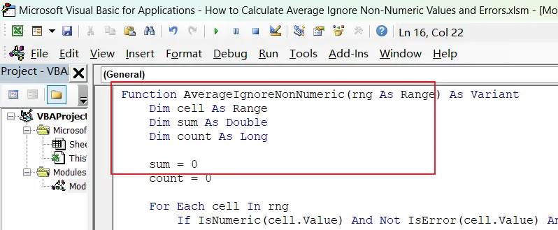
Function AverageIgnoreNonNumeric(rng As Range) As Variant
    Dim cell As Range
    Dim sum As Double
    Dim count As Long
    
    sum = 0
    count = 0
    
    For Each cell In rng
        If IsNumeric(cell.Value) And Not IsError(cell.Value) And Not IsEmpty(cell.Value) Then
            sum = sum + cell.Value
            count = count + 1
        End If
    Next cell
    
    If count > 0 Then
        AverageIgnoreNonNumeric = sum / count
    Else
        AverageIgnoreNonNumeric = CVErr(xlErrNA)
    End If
End Function

Step4: Save the workbook as a macro-enabled workbook by selecting “Excel Macro-Enabled Workbook” from the “Save as type” drop-down menu.

Step5: Close the Visual Basic Editor and return to the Excel worksheet.

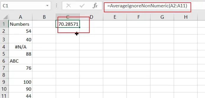
Step6: Enter the below formula in a blank cell where you want to calculate the average

=AverageIgnoreNonNumeric(A2:A11)

Step7: Press “Enter” to calculate the average ignoring non-numeric values.

4. Related Functions

Excel AVERAGE function
The Excel AVERAGE function returns the average of the numbers that you provided.The syntax of the AVERAGE function is as below:=AVERAGE (number1,[number2],…)….
Excel AVERAGEIF function
The Excel AVERAGEAIF function returns the average of all numbers in a range of cells that meet a given criteria.The syntax of the AVERAGEIF function is as below:= AVERAGEIF (range, criteria, [average_range])….

ExcelHow