In Excel there are a lot of built-in functions, and AVERAGE is one of the most frequently used functions. We can apply it to calculate the average of numbers from a given range reference. In daily work, we may apply AVERAGE function together with some other functions to get average based on some conditions. For example, get the average of sales in the nearest 3 days. In this article, we will let you know the method to apply AVERAGE function together with OFFSET function and COUNT function to get the average of last N values from a dynamic range.

In this article, we will introduce you the syntax, arguments, and basic usage of above three functions. We will also explain how the formula works with these functions.

1. Average the Last N Values using Formula

a. EXAMPLE

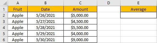
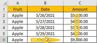
In this case, we want to calculate the average of the last 3 values in “Amount” column. If “Amount” range is a fixed range, we can directly create formula “=AVERAGE(C4:C6)” to get the average of last 3 values. If this range is a dynamic range, for example add a new line for date 5/31/2021, the last 3 values are changed due to a new row is inserted. So, the simple formula with only AVERAGE function doesn’t work.

To get the average of last N values for a dynamic range, we can apply AVERAGE function together with other functions to help us. In this article, to approach our goal, we also apply OFFSET function together with COUNT function to help us set our average range.

b. FORMULA with AVERAGE & OFFSET & COUNT FUNCTIONS

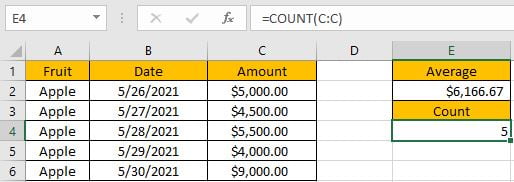
In E2, enter the formula:

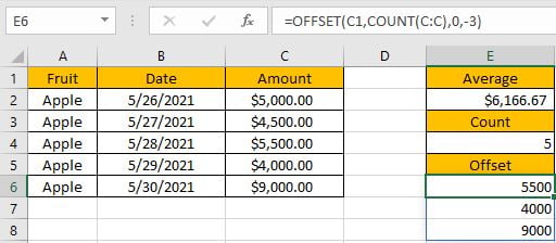
=AVERAGE(OFFSET(C1,COUNT(C:C),0,-3))

Then press Enter, average of last three amounts is $6166.67.

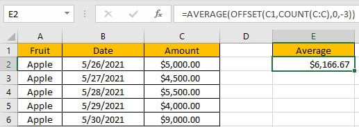
(5500+4000+9000)/3=6166.666666, keep two decimal places 6166.67. The formula works correctly.

c. FUNCTION INTRODUCTION

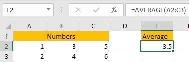
AVERAGE function returns the average of numbers from a given range reference.

Syntax:

=AVERAGE(number1, [number2], …)

Usage:

OFFSET returns a number or a dynamic range based on given five parameters: starting point, row offset, column offset, height in rows and width in rows.

Syntax:

=OFFSET(reference, rows, cols, [height], [width])

Usage 1:

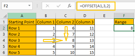
Reference: A1, it is the starting point

Rows: 3, 3 rows below the starting point

Cols: 2, 2 columns to offset to the right of the starting point

Height & Width: optional, no value

Usage 2:

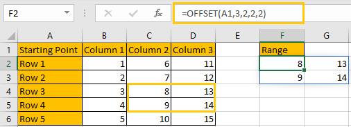
Reference: A1, it is the starting point

Rows: 3, 3 rows below the starting point

Cols: 2, 2 columns to offset to the right of the starting point

Height: 2, it is used together with width, determine the size of the returned range reference, in this case is 2*2 (two rows*two columns)

Width: 2, it is used together with height, determine the size of the returned range reference, in this case is 2*2 (two rows*two columns)

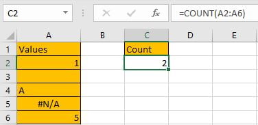
COUNT returns the count of numbers from a given range.

Syntax:

 =COUNT(value1, [value2], …)

Usage:

d. EXPLANATION

=AVERAGE(OFFSET(C1,COUNT(C:C),0,-3))

In this formula, C:C is a full column reference, it represents the entire C column; if user want to cover entire C, D and E columns, we can enter C:E to represent multiple columns, just enter the start column index and end column index, use colon “:” to concentrate them. A full row reference is similar with a full column reference, for example, 1:3 means the first three entire rows. We often use full column or row reference when the selected range is a dynamic range, and user may add or delete column or row at any moment.

In this case, COUNT(C:C) returns 5, there are five cells with numbers in column C.

Now, for OFFSET part, the five inputs are:

Reference: C1 (header of column C, it will not be included when counting row and columns)

Rows: 5. 5 rows below the starting point. The returned range is started in row 6.

Cols: 0. No column to offset to the starting point.

Based on above “Rows” and “Cols” two parameters, we can confirm one point of our returned range, it is C6.

Height: -3. It represents that the returned range is 3 rows in height. Currently, Excel OFFSET function can handle the case height and width are negative numbers. In this case, height value is “-3”, so from C6, OFFSET function expands the range 3 rows backwards to the starting point C1.

Width: No value. Width value is optional for OFFSET function. If it is omitted, the returned range is only limited in current column.

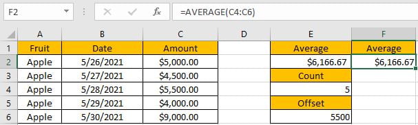
Based on above “Height” and “Width”, we can confirm the returned range, it is C4:C6.

Now, =AVERAGE(OFFSET(C1,COUNT(C:C),0,-3)) is equal to =AVERAGE(C4:C6). After above steps, we get correct value 6166.67.

2. Average the Last N Values with VBA Code

If you want to average the last N values in Excel using a user-defined function with VBA code, you can follow these steps:

Step1: Press ALT+F11 to open the Visual Basic Editor.

Step2: In the Visual Basic Editor, select Insert > Module to create a new module.

Step3: Paste the following code into the module:

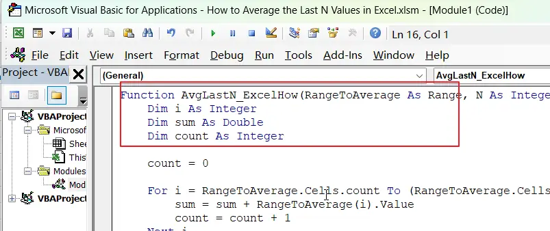
Function AvgLastN_ExcelHow(RangeToAverage As Range, N As Integer) As Double
    Dim i As Integer
    Dim sum As Double
    Dim count As Integer
    
    count = 0
    
    For i = RangeToAverage.Cells.count To (RangeToAverage.Cells.count - N + 1) Step -1
        sum = sum + RangeToAverage(i).Value
        count = count + 1
    Next i
    
    AvgLastN_ExcelHow = sum / count
End Function

Step4: Save the module and close the Visual Basic Editor.

Step5: Type the following formula into a blank cell.

=AvgLastN_ExcelHow(C2:C6,3)

Where C2:C6 is the range of cells that you want to average, and 3 is the number of values you want to include in the average.

Step6: Press Enter to calculate the average.

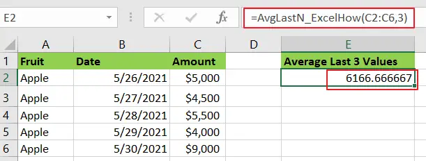
This custom function will calculate the average of the last 3 values in the specified range.

3. Video: Average the Last N Values

This video will demonstrate how to use a formula and VBA code to calculate the average of the last N values in Excel.

4. Related Functions

• Excel AVERAGE function
  The Excel AVERAGE function returns the average of the numbers that you provided.The syntax of the AVERAGE function is as below:=AVERAGE (number1,[number2],…)….
• Excel COUNT function
  The Excel COUNT function counts the number of cells that contain numbers, and counts numbers within the list of arguments. It returns a numeric value that indicate the number of cells that contain numbers in a range…