This post will guide you how to search and highlight multiple values of a apecific value in excel. How to check if a number is a multiple of a specific number and then highlight those searched values in excel.
Table of Contents
Highlight Multiples of Specific Value
If you want to highlight numbers that are multiples of a specific number, and you need to find those numbers firstly and then you can use the conditional formatting feature to highlight it. You need to create a formula based on the MOD function.
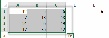
Assuming that you want to highlight multiples of a specific number 6 in Cell E1, Just do the following steps:
#1 select the range of cells A1:C4
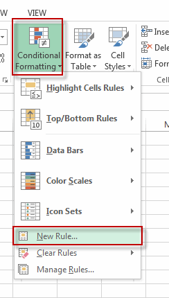
#2 go to Home tab, click Conditional Formatting command under Styles group, and select New Rule…menu from the drop down menu list. The New formatting Rule dialog box will appear.
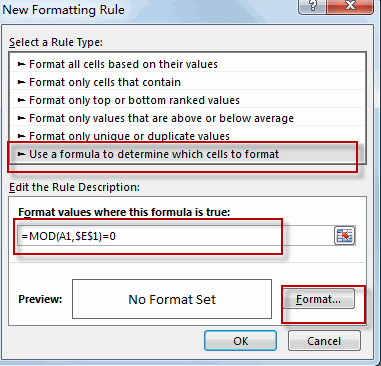
#3 select Use a formula to determine which cells to format in the Select a Rule Type: section. And enter the formula =MOD(A1,$E$1)=0 into the Format values where this formula is true: text box, then click Format…. button. The Format Cells window will appear.
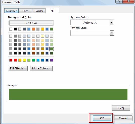
#4 switch to the Fill tab, select one background color that you want to highlight. Then click OK.
#5 click OK button.
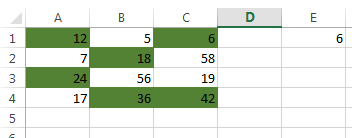
Note: Conditional formatting is used to evaluate for each cell in the selected range with the MOD function to check the remainder of dividing the value in each cell, if the remainder is zero, the value should be an even multiple of the specific number.
Related Functions
- Excel MOD function
he Excel MOD function returns the remainder of two numbers after division. So you can use the MOD function to get the remainder after a number is divided by a divisor in Excel. The syntax of the MOD function is as below:=MOD (number, divisor)….
Leave a Reply
You must be logged in to post a comment.