This tutorial will guide you how to use nested Google Sheets IF function  (include multiple If statements in Google Sheets formula) with syntax and provide about 15 nested IF formula examples with the detailed explanation in Google Spreadsheets.

Description

The Google Sheets IF function perform a logical test to return one value if the condition statement is TRUE and return another value if the condition statement is FALSE. The IF function is a build-in function in Google Spreadsheets and it is categorized as a Logical Function.

The Google Sheets if function just only test one condition and if you want to deal with more than one condition and return different actions depending on the result of the tests,  then you need to include several IF statements (functions) in one Google Sheets IF formula, these multiple IF statements are also called Google Sheets Nested IF formula(Nested IFs). It’s also similar with IF-THEN-ELSE statement.

The nested IF function is formed by multiple if statements within one Google Sheets if function. This Google Sheets nested if statement makes it possible for a single formula to take multiple actions.

Syntax

The syntax of Nested IF function is as below:

=IF(Condition_1,Value_if_True_1,IF(Condition_2,Value_if_True_2,Value_if_False_2))

Where the Nested IF function argument is:

• Condition_1 –  The condition that you want to test  in the first IF statement.
• Value_if_True_1 – The value that is returned if first IF statement is True. If the condition_1 return False, then move into the next IF function.
• Condition_2 – The condition that you want to test in the second IF statement.
• Value_if_True_2 – The value that is returned if second IF statement is True.
• Value_if_False_2 – The value is returned if second IF statement is False.

This is equivalent to the following IF THEN ELSE statement:

IF Condition_1 THEN
    Value_if_True_1
ELSEIF Condition_2
    Value_if_True_2
ELSE
    Value_if_False_2
END IF

Examples of Nested IF function (Statement) in Google Sheets

The below examples will show you how to use Google Sheets Nested IF function with the detailed explanation of their syntax and logic.

Example 1#  The most basic Nested IF function with one level of nesting

If you want to write a nested if function to test the following calculation logic for assigning value in the cell A1.

IF A1 =="excelhow" THEN
    return "Google Sheets "
ELSEIF A1 == "excelhow.net" THEN
    return "Google Spreadsheets "
ELSE
    return "GS"END
 IF

we can write a nested IF function based on the above logic as follows:

=IF(A1="excelhow", "Google Sheets", IF(A1="excelhow.net"," Google Spreadsheets","GS"))

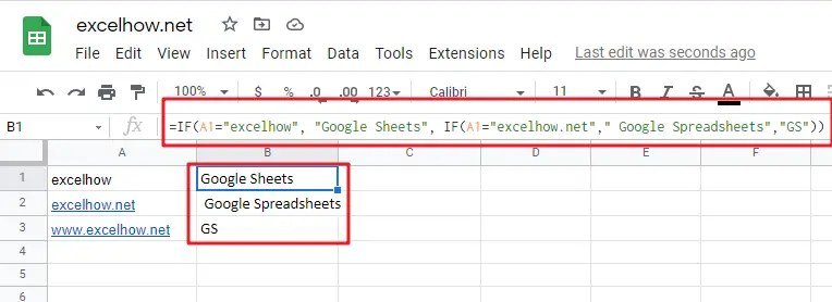
In above Nested IF formula, the nested if function is is inside the outer IF function. we can see that if A1 is not equal to the “excelhow“, then the second nested  IF function will be test. and if second IF condition statement return FALSE, then the entire IF function will return “GS” value.

Example 2#  The Nested IF function with two levels of nesting

Assuming that you want to test more than one condition statement in the above nested if function, add one condition to test if the value of the cell A1 reference is equal to “www.excelhow.net” , If TRUE, then return “google spreadsheets “.

The calculation Logic is as below:

IF A1 =="excelhow" THEN
    return "google"
ELSEIF A1 == "excelhow.com" THEN
    return "google sheets"
ELSEIF A1 == "www.excelhow.net" THEN
    return "google spreadsheets"
ELSE    return "gs"
END IF

we can add one more IF statement inside the second IF function in the above google sheets nested if formula in example1. let’s see the below nested if function with tow level nesting:

=IF(A1="excelhow", "google", IF(A1="excelhow.com"," google sheets",IF(A1="www.excelhow.net","google spreadsheets","gs")))

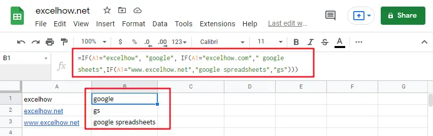
In the above nested google sheets IF formula, the first nested if function is marked with red color, and the second nested google sheets if function is marked with blue color.

If the both first and second conditions are False and the third IF condition will be check, IF A1 is equal to “www.excelhow.net” , then return “google spreadsheets “, or the entire nested IF formula will return “gs“.

Example 3#  Describes the each IF function contained in the nested IF function

​We will use one typical example of google sheets nested if function to describe each IF function included in the nested if function.

Assuming that you need to assign a grade based on a score with the following test conditions:

Score	Grade
80-100	excellent
60-79	good
0-59	bad

Let’s write a nested if function based on the above logic as follows:

=IF(A1>=80, "excellent", IF(A1>=60, "good", IF(A1>0, "bad", "no valid score")))

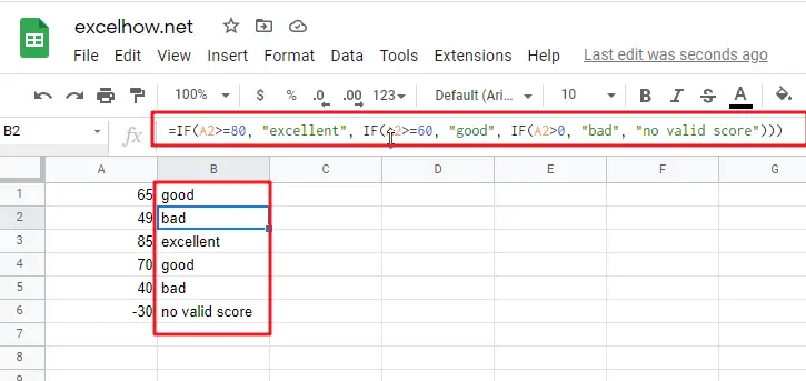
For the above google sheets if formula, lets describe it for each IF function statement.

1# IF Cell A1 is greater than or equal to 80, then the formula will return “excellent” or move to the second If function.

2# If Cell A1 is greater than or equal to 60, then the formula will return  “good” or move to the third IF function

3# IF Cell A1 is greater than 0, then the formula will return “bad”, or the IF function will return “no valid score”.

Example 4#  Describes each If function in the google sheets Nested IF Statement (another simple example of if function)

Let’s describe the below Nested IF Function example:

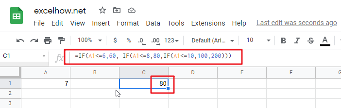
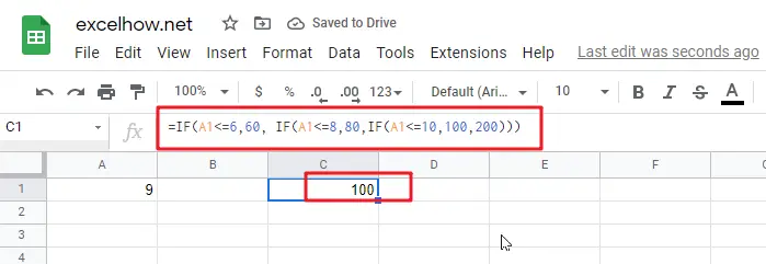
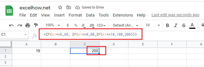
=IF(A1<=6,60, IF(A1<=8,80,IF(A1<=10,100,200)))

a) If cell A1 is equal to 6 or less than 6, then return value 60 in cell C1. Let’s see below screenshot.

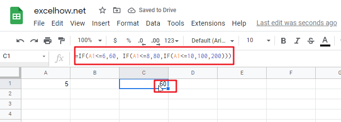
b) If Cell A1 is greater than 6 and less or equal to 8, then retrun value 80 in Cell C1.

c) If cell A1 is greater than 8 and less than or equal to 10, then return value 100 in cell C1.

d) If cell A1 is greater than 10 , then the Nested if function will return the last value “200”in cell C1.

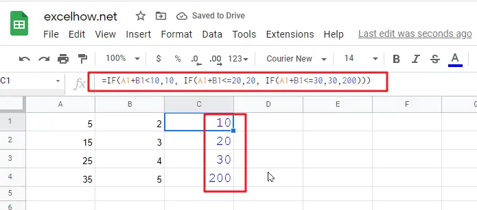
Example 5#  Google Sheets Nested IF function with arithmetic operator (+, -, * , /)

Assuming that you want to write a Nested If function to reflect the following logic tasks:

a) IF Cell A1 is less than 10, then multiply by 10.

b) IF Cell A1 is greater than or equal to 10 but less than 20, then add 20

c) IF Cell A1 is greater than or equal to 20 but less than 30, then minus 20

d) IF Cell A1 is greater than or equal to 30 but less than 50, then divided by 20

The nested IF formula is as follows:

=IF(A1<10,A1*10,IF(A1<20,A1+20,IF(A1<30,A1-20,IF(A1<50,A1/20))))

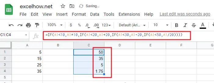
a1) if Cell A1 is less 10 (A1=5), then the first If condition matched and will take multiply action, A1 * 10=5*10=50, so it will return 50 in the cell C1

b1) if Cell 10<=A1<20 (A1=15), then the second if condition matched and will take add action, A1+20=15+20=35, so it will return 35 in the cell C1.

c1) if Cell 20<=A1<30(A1=25), then the third if condition matched and will take minus action, A1-20=25-20=5, so it will return 5 in the cell C1.

d1) if Cell 30<=A1<50 (A1=35), then the forth if condition matched and will take divide action, A1/20=35/20=1.75, so it will return 1.75 in the cell C1.

Example 6#  Google Sheets Nested IF function with logical function –AND

Assuming that you need a nested if function to reflect the following logic:

a) IF A1+B1 is less than 10, then return 10

b) IF A1+B1 is greater than 10 but less than or equal to 20, then return 20

c) IF A1+B1 is greater than 20 but less than or equal to 30, then return 30.

d) IF A1+B1 is greater than 30, then return 200.

Let’s write the following nested IF formula in the cell C1:

=IF(A1+B1<10,10, IF(A1+B1<=20,20, IF(A1+B1<=30,30,200)))

The above formula just use basic nested IF function syntax, we also can use logic function to re-write it, the nested if formula with AND function is as follows:

=IF((A1+B1)<10,10,IF(AND((A1+B1)>10,(A1+B1)<=20),20, IF(AND((A1+B1)>20,(A1+B1)<=30),30,200)))

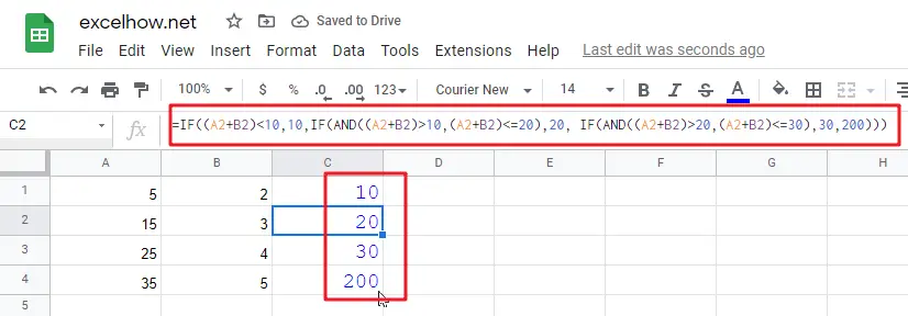
The above nested IF formula combined with two AND function.

In the second IF Statement, AND((A1+B1)>10,(A1+B1)<=20) will check if 10<A1+B1<=20, If TRUE, then the formula will return 20.

In the third IF Statement, AND((A1+B1)>20,(A1+B1)<=30) will check if 20<A1+B1<=30, If TRUE, then the formula will return 30.

Example 7# Google Sheets Nested IF function with logical function –OR

Assuming that you need a nested if function to reflect the following logic:

a) IF Cell A1=5, return A1/B1

b) IF Cell A1=10, return A2/B2

c) IF Cell A1=15 or A1=20, return A3/B3

In Cell C1, we can write the below nested if formula based on the above conditions.

=IF(A1=5,A1/B1,IF(A1=10,A2/B2,IF(OR(A1=15,A1=20),A3/B3)))

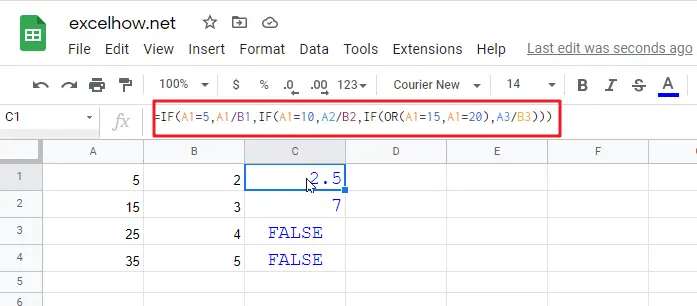
One OR function be used in the above excel nested if function, it will check if A1=15 or A1=20, if TRUE, then return A3/B3.

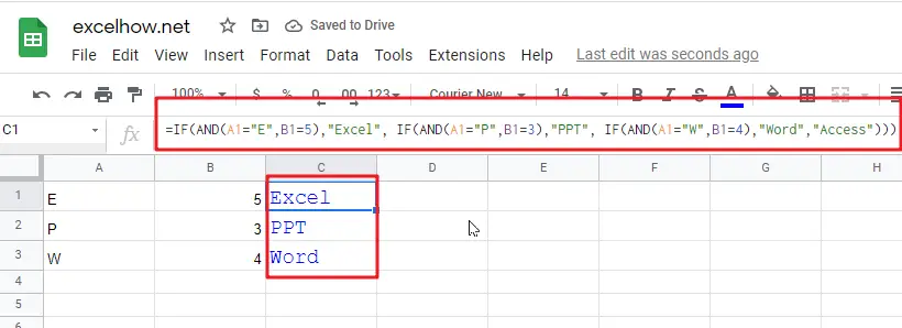
Example 8#  Google Sheets nested if function with text and logical function AND

Wrote a nested if function with text to reflect the following logic:

a) If Cell A1=”E” and Cell B1=5, then return “Excel”

b) If Cell A1=”P” and Cell B1=3, then return “PPT”

c) If Cell A1=”W” and Cell B1=4, then return “Word”

d) Else return “Access”

In Cell C1, try to enter into the following excel nested If formula with AND function:

=IF(AND(A1="E",B1=5),"Excel", IF(AND(A1="P",B1=3),"PPT", IF(AND(A1="W",B1=4),"Word","Access")))

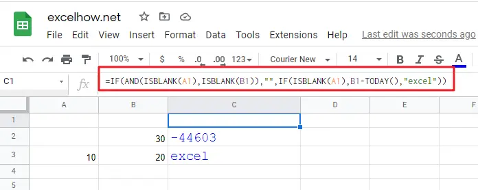
Example 9#  Google Sheets nested if function with ISBLANK function and logical function AND

a) If you want to wrote a nested if function with ISBLANK function and logical function AND to reflect the following logic:

b) If both Cell A1 and Cell B1 are empty, then return “”

c) If only Cell A1 is empty, then return B1-today()

d) If both two cells A1 and B1 are not empty, then return “excel” string.

In Cell C1, use the following excel nested If formula with ISBLANK and AND function:

=IF(AND(ISBLANK(A1),ISBLANK(B1)),"",IF(ISBLANK(A1),B1-TODAY(),"excel"))

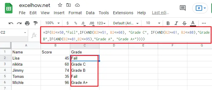
Example 10#  Using nested IF functions to check grade level based on student’s score(multiple IF statements)

The logic is as below:

Scores	Grade
<50	Fail
51 to 60	Grade C
61 to 80	Grade B
81 to 95	Grade A
96 to 100	Grade A+

We will write a nested If function that reflect the above logic, and will check if the score is below 50, If TRUE, it is considered as “Fail”. If FALSE, move into the next IF statement to test if the score is between 51 and 60 and it is considered as “Grade C”. If False, we will move into another IF statement to check if the score is between 61 and 80, IF True and it is considered as “Grade B”. If FASLSE, just check the rest conditions.

We can use a nested if formula as follows:

=IF(B2<=50,"Fail",IF(AND(B2>=51, B2<=60), "Grade C", IF(AND(B2>=61, B2<=80),"Grade B",IF(AND(B2>=81,B2<=95),"Grade A", "Grade A+"))))

Example 11#  Nested IF function for checking two Empty Cells

Let’s see the below image a product table of a company (need to create a Google sheets table firstly):

a) If we need to check both “Price” cell and “Quantity” cell are empty, If True, then return empty. If the only “price” cell is empty only, IF True, return empty.

b) If the only “Quantity” cell is empty, IF True, return empty.

c) If both “price” and “Quantity” are not empty, then return multiply Price * Quantity as subtotal value.

So To check both “Price” and Quantity cells, we can use table header name as condition variable to test each Price cells or Quantity cells, so we can write the nested if formula as follows:

=IF([Price]="","",IF([Quantity]="","",[Price]*[Quantity]))

Just using the above Google sheets if formula in the subtotal cells, the formula will check the first IF statement if Price Cell is empty, IF TRUE, then will return empty (“”) in the subtotal cell. IF FALSE, then move to the next IF statement and so on. Last, IF neither cell is empty, then will return the value of multiply [Price]*[Quantity] in subtotal cell.

Of course, we can use another nested if function to achieve the above calculation logic (easy to understand).

=IF(ISBLANK(B2),"",IF(ISBLANK(C2),"", B2*C2))

OR

=IF(B2="","",IF(C2="","", B2*C2))

Nested IF Functions Order

There is one important thing that need us keep in mind when write Google sheets Nested IF Function, it is the order of nested IF function. It can nested up to 64 If statements, and how to order multiple IF condition statements, it is key point. Or the wrong result will be returned. The point is that Google sheets nested if function will test the first if condition in the order, once any condition is met, and the subsequent if conditions will not be checked.

So let’s remember the below rules while writing Google sheets nested if function:

• The most important condition First or Harder Test First

Let’s see the below example what it means:

Example 12#

There are two test conditions in the following Google sheets nested if function:

=IF(B1>=90,"excellent",IF(B1>=60,"good","bad"))

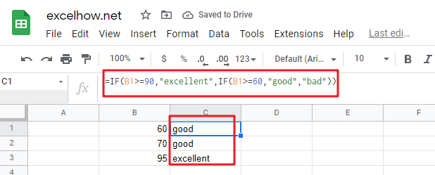
When using this formula in the cell B3, If the amount in cell B1 is 95, then “excellent” would be returned. because it is greater than 90. And the second IF condition will not be evaluated.

However, if the order of nested if statment are reversed as follows:

=IF(B1>=60,”good”,IF(B1>=90,”excellent”,”bad”))

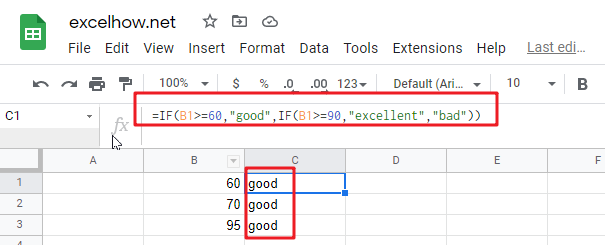
The above formula would check for the condition B1>=60 first, if the amount in cell B1 is 95,  then the value “good” would be returned in cell B3. Because the Cell B1 match the first test condition, and it will not check the second if condition and will return the incorrect result.

Nested IF Function Alternatives

To make your google sheets formulas more efficiency and fast, you can try to use the following alternatives to google sheets nested if function.

1) google sheets nested if function can be easily replaced with the VLOOUP, Lookup, INDEX/MATCH or CHOOSE functions.

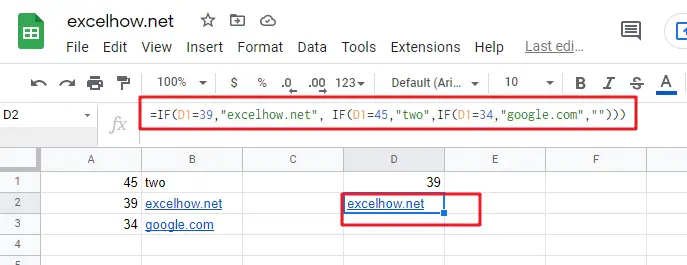
Example 13#  Use VLookup function instead of nested IF function

Nested IF function:

=IF(D1=39,"excelhow.net", IF(D1=45,"two",IF(D1=34,"google.com","")))

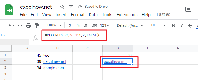
Vlookup function:

=VLOOKUP(39,A1:B3,2,FALSE)

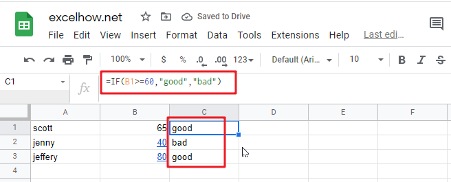
Example 14#  Use CHOOSE function instead of nested if function

Nested If unction:

=IF(B1>=60,"good","bad")

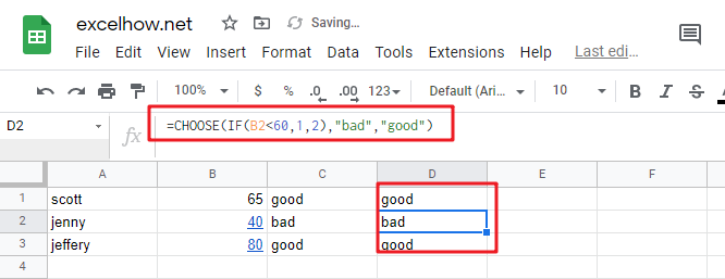
Using CHOOSE function as follows:

=CHOOSE(IF(B1<60,1,2),"bad","good")

2) Use IFS instead of nested if function

3) Use the CONCATENATE function or the concatenate operator (&).

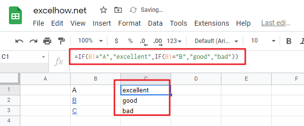
Example 15#

Nested IF function:

=IF(B1=”A”,”excellent”,IF(B1=”B”,”good”,”bad”))

Questions & Asked

Question1: Is there any tool to help write Google Sheets formulas and nested Ifs?

This is a Google Sheets formula with nested IF statements:

=IF((B2="East"),4,IF((B2="West"),3,IF((B2="North"),2,IF((B2="South"),1,""))))

To essentially accomplish this:

If cell B2 = "East"
   return "4"
ElseIf cell B2 = "West"
   return "3"
ElseIf cell B2 = "North"
   return "2"
ElseIf cell B2 = "South"
   return "1"
Else
   return ""

Can Google Sheets formulas be written in such a “more readable” manner and converted to the official syntax? Is there any tool to help write Google Sheets formulas?

Answer:  Google Sheets Formula Formatter add-in by Rob van Gelder, mentioned at Daily Dose of Google Sheets.

Google Sheets formula bar ignores line feeds and white space, so you can Alt+Enter and spacebar to format the formulas however you like. I’ve tried it and I quickly stopped doing it. Too much spacebar-ing, especially if you need to edit.

Question2: I am working on a Google Sheets file, and i am trying to use a nested if formula to achieve what i would like.

i have two columns:A B.  And the condition is this: if the value in a2=a3, then check if the minus of b2 and b3 is certain value, and if it is, put a yes, else put a no. this will iterate till the end of the Google Sheets file.

so far here is what i have. not sure how to use the Google Sheets formulas. any help is much appreciated.

if(a2=a3,b2-b3=5 or b2-b3=-5 or b2-b3=20 or b2-b3=-20, "yes", "no")

Answer: you should be able to use the OR function within your nested if formula to test for “B2-B3=5,B2-B3=-5,B2-B3=20,B2-B3=-20” as follows:

=IF(A2=A3,IF(OR(B2-B3=5,B2-B3=-5,B2-B3=20,B2-B3=-20),"yes","no"),"no")

Related Functions

• Google Sheets ISBLANK function
  The Google Sheets ISBLANK function returns TRUE if the value is blank or null.The syntax of the ISBLANK function is as below:= ISBLANK (value)…

• Google Sheets COUNTIF function
  The Google Sheets CHOOSE function returns a value from a list of values based on index. The syntax of the CHOOSE function is as below:=CHOOSE (index_num, value1,[value2],…) …
• Google Sheets VLOOKUP Function
  The Google Sheets VLOOKUP function lookup a value in the first column of the table and return the value in the same row based on index_num position..The syntax of the VLOOKUP function is as below:= VLOOKUP (lookup_value, table_array, column_index_num,[range_lookup])…
• Google Sheets IF function
  The Google Sheets IF function perform a logical test to return one value if the condition is TRUE and return another value if the condition is FALSE. The IF function is a build-in function in Microsoft Excel and it is categorized as a Logical Function.The syntax of the IF function is as below:= IF (condition, [true_value], [false_value])….
• Google Sheets Choose function
  The Google Sheets CHOOSE function returns a value from a list of values based on index.The syntax of the CHOOSE function is as below:=CHOOSE (index_num, value1,[value2],…)….