This post will guide you how to use Google Sheets VLOOKUP function with syntax and examples.
Table of Contents
Description
The Google Sheets VLOOKUP function lookup a value in the first column of the table and return the value in the same row based on index_num position..
The VLOOKUP function can be used to search down the first column of a range for a key and returns the value of a specified cell in the row found in google sheets. The purpose of this function is to lookup a value in a table by matching on the first column and It’s returned value is the matched value from a table.
The VLOOKUP function is a build-in function in Google Sheets and it is categorized as a LOOKUP function.
Syntax
The syntax of the VLOOKUP function is as below:
= VLOOKUP (lookup_value, table_array, column_index_num,[range_lookup])
Where the VLOOKUP function arguments are:
- Lookup_value -This is a required argument. The value that you want to search for, in the first column of the table. Note: the lookup_value can be a value, a cell or ranges reference, or a text string.
- Table_array – This is a required argument. Two or more columns of data to be searched in the first column.
- column_index_num – This is a required argument. The column number in table_array.
- Range_lookup – This is an optional argument. The value can be set as True or False. If true, the function will return an approximate match value. If False, it will find an exact match or it will return an error value #N/A.
Note:
- If range_lookup is TRUE, VLOOKUP function will match the nearest value less that the lookup_value.
- If range lookup is TRUE, VLOOKUP function will use an exact match if one exists.
- If range_lookup is FALSE, VLOOKUP function will perform an exact match.
- VLOOKUP function is not case-sensitive.
- If you want to search for numeric or data values, you need to make sure that the first column in the range is not sorted by text values.
- When range_lookup is set to TRUE and table_array is sorted, VLOOKUP function has much better performance.
Google Sheets VLOOKUP Function Examples
The below examples will show you how to use google sheets VLOOKUP Function to lookup value from a table or array vertically.
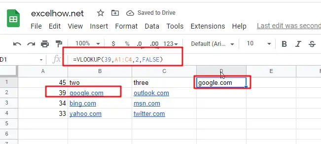
#1 To search “39” text string in the first column and returns the value from column 2 that is in the same row, just using the following VLOOKUP formula:
=VLOOKUP(39,A1:C4,2,FALSE)