This post will guide you how to use Google Sheets IF function with syntax and examples in Google Spreadsheets.
Table of Contents
Description
The Google Sheets IF function perform a logical test to return one value if the condition is TRUE and return another value if the condition is FALSE.
The IF function is a build-in function in Google Spreadsheets and it is categorized as a Logical Function.
Syntax
The syntax of the IF function is as below:
= IF (condition, [true_value], [false_value])
Where the IF function arguments are:
Condition-This is a required argument. A user-defined condition that is to be tested.True_value– This is an optional argument. The value that is returned if condition evaluates to TRUE.False_value– This is an optional argument. The value that is returned if condition evaluates to FALSE.
The below examples will show you how to use Google Sheets IF Function to return one value if the condition is TRUE or FALSE.
=IF(B1>90, "good", "bad")
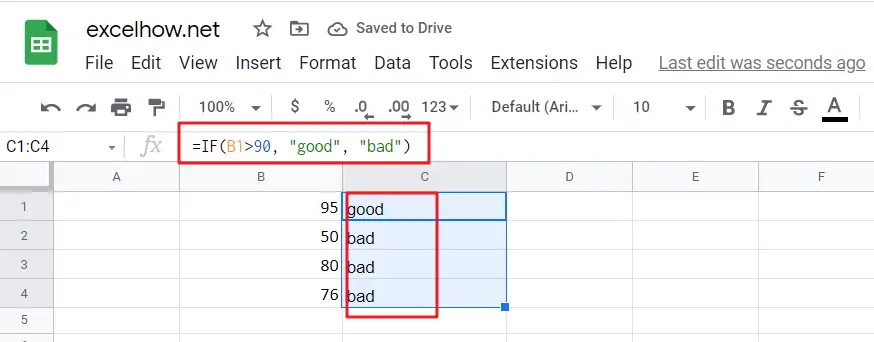
Note: the above Google Sheets formula will test a condition “b1>90”, if the condition is true, then “good” will return or “bad” will return.
Nested IF statements
The Google Sheets IF function just only test one condition and if you want to deal with more than one condition and return different actions depending on the result of the tests, then you need to include several IF statements (functions) in one Google Sheets IF formula, these multiple IF statements are also called Google Sheets Nested IF formula(Nested IFs).
For example:
=IF(A1>=80, "excellent", IF(A1>=60, "good", IF(A1>0, "bad", "no valid score")))
More reading: Google Sheets Nexted IF Functions (Statements) Tutorial
Google Sheets Logical operators
When you are writing an If statement, you may need to use any of the following Google Sheets logical operators:
| Operator | Meaning | Example | Description |
| = | Equal To | A1=B1 | Returns True if a value in cell A1 is equal to the values in cell B1; FALSE if they are not. |
| > | Greater Than | A1>B1 | Returns True if a value in cell A1 is greater than the values in cell B1; FALSE if they are not. |
| >= | Greater Than or Equal to | A1>=B1 | Returns True if a value in cell A1 is greater than or equal to the values in cell B1; FALSE if they are not. |
| < | Less Than | A1<B1 | Returns True if a value in cell A1 is less than the values in cell B1; FALSE if they are not. |
| <= | Less Than or Equal to | A1<=B1 | Returns True if a value in cell A1 is less than or equal to the values in cell B1; FALSE if they are not. |
| <> | Not Equal to | A1<>B1 | Returns True if a value in cell A1 is not equal to the values in cell B1; FALSE if they are not. |
Let’s see some examples for logical operators in Google Sheets formula:
| A1 | B1 |
| 8 | 5 |
  =(A1>B1)  //Output: TRUE

=(A1<B1) //Output: FALSE

=(A1>=B1) //Output: TRUE

=(A1<>8) //Output: FALSE

 =(A1<>B1) //Output: TRUE

 =(IF A1>3, “TRUE”, “FALSE”) //Output: TRUE
Frequently Asked Questions
Question1: I want to write an IF Formula based on the below test criteria in the Google Spreadsheets.
If the number in Cell B1 is greater than 30, then I want it to return A
If the number in cell B1 is between 20 and 30, then I want it to return B
If the number in Cell B1 is below 20, then I want it to return C
The below formula is what I currently write:
=IF(B1>30,"A",IF(B1<30,B1>20,"B","C"))
When I entered the above formula in the Cell C1, and it will return an Error.
Answer: You can use IF function in combination with AND function to reflect the above logic. So you can do it using the following formula:
=IF(B1>30,"A",IF(AND(B1>=20,B1<=30),"B","C"))
Or you can use another IF formula without AND function as follows:
=IF(B1>30,"A",IF(B1<20,"C","B"))
Question 2: I want to write a Google Sheets Formula for sales rep, If the sales are less than 10K, then the member will get no commission. If the sales are between 10 and 50K, then the member will get a 3% commission. If the sales are more than 50k, then the member will get 5% commission. Could you help me?
Answer: Based on the above description, we can use the following Google Sheets IF formula:
=IF(B1<10,0,IF(B1<50,B1*3%,B1*5%))
Question 3: I want to select students for the scholarship in school, and based on the student’s scores and attendance value, if the student scores more than 85 and has the attendance of more than 85%, then he/she will get the scholarship. Please help me how to write this formula based on my test criteria.
Answer: you can use the IF function with the AND function to check whether both of two conditions are met or not. If the test are met, then return “Yes”, otherwise returns “No”.
So you can use the following IF formula in Google Sheets:
=IF(AND(B1>85, C1>85%),"Yes","No")
Question 4: I am trying to write an Google Sheets formula based on the following logic:
I want to enter a formula in Cell C1 that will Add B1, B2 and B3 or multiply B1 by 1, multiply B2 by 2, multiply B2 by 3, which action will be taken based on what you put in Cell D1.
Appreciated for any help. Thanks
Answer: Based on the above logic description, you need to use SUM function to count the sum of B1, B2 and B3. We can use the following IF formula:
=IF(D1="Add”,SUM(B1,B2,B3),IF(D1="Multiply",B1*B2*B3,"ERROR"))
Question 5: I am trying to write a formula in Google Sheets to check the employee number field and returns the relevant band of employee. I already have one IF formula, but I always return the first value of “A”. Could you help?
=IF(B1>=10,"A",IF(B1>=20,"B",IF(B1>=50,"C")))
Answer: when you write an IF nested formula, you need to start with the largest number first or start the smallest number first with less than or equal to operator.
1# start with the largest number first, we can write down the below formula:
=IF(B1>=50,"C",IF(B1>=20,"B",IF(B1>=10,"A")))
2# start with the smallest number first, you need to change the >= to <= , just see the below formula:
=IF(B1<=10,"A",IF(B1<=20,"B",IF(B1<=50,"C")))
Question 6: I want to write a Formula in Google Sheets to return “bad” if the cell B1 is either <100 or >500, otherwise, it should be returned the value of cell B1.
Answer: For the above logic test, we should use the OR function in the IF condition, so we can write down the below IF formula:
=IF(OR(B1>500,B1<100),"good",B1)
Question 7: I want to write a formula in Google Sheets using IF function to check if the cell B1 >10 and B1<20. If TRUE, returns “good”, If FALSE, returns “bad”
Answer: You can use IF function in combination with AND function to check the value of Cell B1, if cell B1 is greater than 10 and cell B1 is less than 20, then returns “good”, otherwise, it will return “bad”.
=IF(AND(B1>10,B1<20),"good","bad")
Question 8: I need to write a nested IF statement in Google Sheets to check the following logic:
If Cell B1 is less than 5, then multiply it by 5.
If Cell B1 is greater than or equal to 5 but less than 10, then multiply it by 10.
If cell B1 is greater than 10, then multiply it by 15.
Answer: This is a generic nested IF formula in Google Sheets, we can write the below nested IF statement to reflect the logic.
=IF(B1<5, B1*5, IF(B1<10, B1*10, B1*15))
Question 9: I want to write a formula to match the following logic in Google Sheets:
If A1*B1 <=10, then returns A
If A1*B1 >10 but A1*B1 <=20, then returns B
If A1*B1 >20 but A1*B1 <=30, then returns C
If A1*B1>30, then returns D
Answer: You can use IF function to build a Nested IF statement in combination with AND function to achieve it. Let’s write down the following IF formula:
=IF(A1*B1<=10,"A", IF(AND(A1*B1>10,A1*B1<=20),"B", IF(AND(A1*B1>20,a1*B1<=30,"C","D"))))
Question 10: I want to write an IF function to check if the value in cell B1 is blank or Text string or Numeric value, if the cell B1 is empty, then return “blank”, if the cell B1 is a text string, then return “Text”, if the value in cell B1 is a numeric value, then return “number”. Any help for this formula, thanks.
Answer: Based on the description, you need to use ISBLANK function to check if the value in cell b1 is blank or not. And need to use ISTEXT function to check if the value in cell B1 is a text string or not and need to use ISNUMBER function to check if the value in cell B1 is a number or not. So you can write a nested IF statements in combination with ISBLANK, ISTEXT and ISNUMBER functions in Google Sheets as follows:
=IF(ISBLANK(B1),"blank", IF(ISTEXT(B1),"Text", IF(ISNUMBER(B1),"number")))
Question 11: I want to write a formula in Google Sheets to calculate the bonus for employees in company, if the employee salary is greater than or equal to $2000, then the bonus will be 10% of the salary , otherwise, the bonus will be 5% of the employee salary.
Answer: we need to check if the salary in Cell B1 (it’s the salary of the first employee) is greater than or equal to 2000. It the condition test is TRUE, then returns B1*10%, otherwise returns b1*5%. So we can write down the following IF formula in Google Sheets:
=IF(B1>=2000, B1*10%, B1*5%)
Question 12: In Google Spreadsheets, I want to create an IF function to check if any employee who have at least 10 years of experience and whose salary is greater than $5000, If TRUE, then the bonus will be 20% of salary.
Answer: you can use IF function in combination with AND function to check if the value in cell B1 is greater than or equal to 10 and the value in Cell C1 is greater than 5000. If both of two conditions are TRUE, then returns C1*20%, otherwise returns “No Bonus”.
Let’s write down the following IF statement as follows:
=IF(AND(B1>=10,C1>5000),C1*20%, "No Bonus")
Question 13: I want to create an IF formula in Google Sheets to check the following text logic:
If B1<10, then multiply B1 by 1%, but the returned value is not less than 50.
If B1>10, then multiply B1 by 2%, but the returned value is not greater than 100.
Answer: To reflect the first test condition, you need to use MAX function to match the condition. To reflect the second test condition, you need to use MIN function to match that the returned value should not be greater than 100. So we can use the following Google Sheets IF formula:
=IF(B1<10, MAX(50,B1*1%), IF(B1>10, MIN(100,B1*5%)))
Question 14: I want to use IF function to check if B1 is greater than 10 and B2 is greater than 20 and B3 is less than 30, if TRUE, then returns “good”, otherwise, it should be returned “bad”. So How to create the IF formula based on the above test criteria to check three conditions at the same time.
Answer: you need to use AND function within the IF function in Google Sheets to create an IF formula as follows:
=IF(AND(B1>10,B2>20,B3<30),"good","bad")
Question 15: I have an IF formula that might cause a division by zero error, I don’t know how to avoid this kind of errors in Google Sheets formula.
Answer: You can use ISERROR function to catch this kind of errors then use the IF function to check the returned values from ISERROR function to avoid an error. So we can write an IF function in combination with ISERROR function in Google Sheets. For example, we can use the following IF formula:
=IF(ISERROR(B1/C1),0, B1/C1)
The ISERROR function will return TRUE when trying to divide B1 by 0.
Question 16: I need to create a formula in Google Sheets to reflect the following logic:
If B1=Google, then return E
If B1=sheets, then return W
If B1=info, then return A
Answer: You can use IF function to create a nested IF statements as follows:
=IF(B1=" Google ","G",IF(B1=" sheets ","S",IF(B1=" info ","I")))
Question 17: I have a worksheet that containing cells that are formatted as date format. I want to write an IF formula to check the first value in Cell (month part). So I am trying to create the following IF formula:
=IF(LEFT(B1,1)=8, "August","Null")
The returned results are always “Null”.
Answer: As the dates are not recognized as string, so you cannot use the LEFT function to exact the first value in the dates. At this moment, you need to use Month function to convert the date to its month number in Google Sheets. So we can write down the below IF formula in combination with Month function:
=IF(MONTH(B1)=8, "August","Null")
Question18: I am trying to create an IF formula to check if the time value in cells are greater than 10.00h for the following date format: 08/11/2018 09:43.50. Appreciative of any help.
Answer: In Google Sheets, you can use HOUR, MINUTE, SECOND functions to compare the date or time value. so if you want to compare the value in Cell B1 if it is greater than 10h, then you can use HOUR function within IF function, just like this: HOUR(B1)>10, so we can write down the below formula:
=IF(HOUR(B1)>10, "greater","less")
Question 19: I want to create an IF function and need to combine with another RAND function. The formula just works find for the first IF_VALUE_TRUE statement, but the formula works not good for IF_VALUE_FALSE statement. Here is the IF formula I have got:
=IF(ISBLANK(B1),"","=rand()")
In the above IF function, it will return empty string when the value in cell B1 is blank. Otherwise, it should add a random function, the problem is that the cell doesn’t run the RAND function. So how can I fix it? Thanks
Answer: when you write an IF formula, if you want to enclose others function, you need not to add quotes around the RAND () function, so just remove the quotes and equal sign in your IF function. Just like the below IF formula:
=IF(ISBLANK(B1),"",RAND())
Question 20: I am trying to write an IF formula in Google Sheets to reflect the following logic:
If B1 is greater than or equal to 50 and C1 is 0
OR
If B1 is greater than or equal to 30 and C1 is greater than or equal to 1
OR
If B1 is greater than or equal to 20 and C1 is 2
Then take the following action: D2/E2
Otherwise, return FALSE
I have wrote the following IF formula, but it doesn’t work at all.
=IF(AND(B1>=50,C1>=0),OR(AND(B1>=30,C1>=1)),OR(AND(B1>=20,C1>=2)),D2/E2,"FALSE")
Answer: you need to nest your different AND function within an OR function in the IF formula. So you can try the below IF formula:
=IF(OR(AND(B1>=50,C1>=0),AND(B1>=30,C1>=1),AND(B1>=20,C1>=2)), D2/E2,"FALSE")
Question 21: I want to create an IF function in combination with MID function in Google Sheets. it need to check if the value in one specified cell is TRUE, then return the first six characters from another cell. Otherwise return empty value.
Answer: you just need to add MID function within IF function in Google Sheets, and do not add any quotes around MID function. So you can use the following IF formula to achieve your request:
=IF(B1=TRUE, MID(C1,1,5), "")
Question 22: I have a Google Sheets as below:
A B
——
20 O
30 V
10 T
50 T
I want to create an IF formula to reflect the following logic:
IF cell A1 is less than or equal to 30 and Cell B1 is equal to “O” or “V”, if TRUE, then returns 300, otherwise returns 400.
IF Cell A1 is greater than 30 and Cell B1 is equal to “O” or “V”, then returns 500, otherwise returns 600.
I have wrote the below tow IF formulas for the above two conditions as follows:
=IF(AND(A1<=30,OR(B1="O",B1="V")),300,400)

=IF(AND(A1>30,OR(B1="O",B1="V")),500,600)
I am able to check the above two IF formula and the returned results is OK… But I am not able to combine the above two IF formula into a single IF formula. So anybody can help? Many thanks
Answer: Based on the above logic, you can use the below IF formula to combine with above two IF formulas:
=IF(A1<=30,IF(OR(B1="O",B1="V"),300,400),IF(OR(B1="O",B1="V"),500,600))
Question 23: I am trying to write an IF function to prevent zero and negative values in cells. What I would like is that if the value in cell B1 is less than or equal to 0, then it should be returned “Null” otherwise, it should return the calculation of Cells value, like as:B2*(C2-D2)*E2.
The below IF formula is what I have:
=IF(B1<=0,"Null","B2*(C2-D2)*E2")
When I run the formula above, it only returns my calculation string and do not take the actual calculation.
Answer: In Google Sheets, the double quotes make any values in between be recognized as Text string. So if you want to take calculation for your IF formula, just remove the double quotes. Let’s see the modified IF formula as follows:
=IF(B1<=0,"Null",B2*(C2-D2)*E2)
Question 24: I want to create an new IF function to check if the value in cells is Saturday or Sunday, If TRUE, returns “yes”, otherwise, returns “No”. And I am using the following IF formula, but I get an error, so what’s wrong for this formula?
=IF((OR($B1="Saturday","$B1="Sunday"),"yes","no"))
Answer: you need to use the WEEKDAY function within IF function to handle the dates if they are in date format, like as: 11/8/2018.
So you can use the below IF function to achieve your logic:
=IF(WEEKDAY($B$1,2)>5,"yes","no")
You can also use TEXT function within the IF function to achieve the same results, just like the below IF formula:
=IF(LEFT(TEXT($B$1,"ddd"))="S","yes","no")
Question 25: I want to write an IF function in Google Sheets to check if the first character in one Cell is equal to 5, then the returned value should be the five rightmost characters of that cell, otherwise, the returned value should be the four rightmost characters. I wrote one IF formula as follows, but it doesn’t work.
=IF(LEFT(B1,1)=5, RIGHT(B1,5),RIGHT(B1,4))
In the above IF function, it always return the rightmost four characters even though the first character in Cell B1 starts with “S”. Please help me to fix it.
Answer: you should know the returned value of the LEFT function firstly in Google Sheets. As the LEFT function will return a Text value, so you also need to provide a string for comparison, so adding quotes to enclose it. Just like the below IF function:
=IF(LEFT(B1,1)="5", RIGHT(B1,5),RIGHT(B1,4))
There is another way to achieve the same results, you can use NUMBERVALUE function to convert the result of LEFT function to a numeric value, like the below IF function:
=IF(NUMBERVALUE(LEFT(B1,1))=5,RIGHT(B1,5),RIGHT(B1,4))
Question 26: I have 2 columns contain date and time or just only contain time. And I want to check if the times of column A is greater than the times of column B. the key issue may be that column A has the date and time. I wrote the following IF formula to run it in Cell C1, but it returned the inaccurate results.
=IF(A1>B1,"yes","no")
Any help would be appreciated… Many thanks!
Answer: the date part of the value in column A is the integer, while the time is the decimal. You can use the following IF formula:
=IF(A1-INT(A1)>B2),"yes","no")
Question 27: The below are the results that I expected, and I want cell B1 to B4 can detect the string from A1 to A4 automatically and return the same string value plus the severity level when the test match. For example, If A1 is equal to “critical”, then it should be returned “critical severity 1” in the cell B1. Etc.
And I am using the following IF formula, but it does not work at all. Please help to fix it. Thanks
=IF(A1="Critical","Critical Severity 1",""),IF(A1="High","High Severity 2",""),IF(A1="Medium","Medium Severity 3",""),IF(A1="Low","Low Severity 4","")
| A | B |
| critical | critical severity 1 |
| high | high severity 2 |
| medium | Medium severity 3 |
| low | low severity 4 |
Answer: you can try to run the following IF formula in Google Sheets:
=IF(A1="critical","critical Severity 1",IF(A1="high","high Severity 2",IF(A1="medium","medium Severity 3",IF(A1="low","low Severity 4",""))))
Question 28: I am working on a Google Sheets file and want to create a new IF formula to reflect the following logic:
If the value in Cell A1 is equal to the value in Cell A2, then check if the minus of B1 and B2 is equal to a special value, and if the condition is TRUE, returns “yes”, otherwise, returns “no”. Here is the IF formula I have:
=if(A1=A2,B1-B2=5 or B1-B2=-5 or B1-B2=20 or B1-B2=-20, "yes", "no")
Any help is appreciated…Thanks
Answer: you need to use OR function with IF function to create a nested IF statement to achieve your request. So you can try the following Google Sheets IF formula in your Google Sheets file.
=IF(A1=A2,IF(OR(B1-B2=5,B1-B2=-5,B1-B2=20,B1-B2=-20),"yes","no"),"no")
Question 29: I want to create an IF formula to check the range of cells in Google Sheets. I have scores of different subject for a student, and want to check if any one of scores is less than 60, If TRUE, then return “BAD”. Can this logic be done with the IF statements in Google Sheets?
Answer: you can use COUNTIF function within IF function to create a generic IF formula as follows:
=IF(COUNTIF(B:B,"<60")>0,"BAD","Good")
Question 30: I am trying to create a new IF statement so that when the formula is looking at Row A and Row B, the returned values should be shown in the Row C. the following logic need to be checked:
IF the value in the Row A is equal to “NA” And the value in the Row B is equal to “NA”, then return “NA” value in Row C.
IF the value in the Row A is equal to “NA”, and the value in the Row B is equal to “denied”, then return “denied” value in Row C.
IF the value in the Row A is equal to “allowed” and the value in the Row B is equal to “NA”, then return “allowed” value in Row C.
Here is my formula:
=IF(AND(A1 = "NA", B1 = "NA"),"NA",IF(OR(A1="denied",B1 ="denied"),"denied", "NA"))
I don’t know how to include “allowed” in the IF formula above, anyone can help this, many thanks.
Answer: This is a typical nested if statement, you can use OR function within IF function in Google Sheets. We can write down this nested IF formula as follows:
=IF(OR(A1="denied", B1="denied"), "denied", IF(OR(A1="allowed", B1="allowed"), "allowed", "NA"))
Related Functions
- Google Sheets ISBLANK function
The Google Sheets ISBLANK function returns TRUE if the value is blank or null.The syntax of the ISBLANK function is as below:= ISBLANK (value)…
- Google Sheets COUNTIF function
The Google Sheets CHOOSE function returns a value from a list of values based on index. The syntax of the CHOOSE function is as below:=CHOOSE (index_num, value1,[value2],…) … - Google Sheets IF function
The Google Sheets IF function perform a logical test to return one value if the condition is TRUE and return another value if the condition is FALSE. The IF function is a build-in function in Microsoft Excel and it is categorized as a Logical Function.The syntax of the IF function is as below:= IF (condition, [true_value], [false_value])…. - Google Sheets LEFT function
The Google Sheets LEFT function returns a substring (a specified number of the characters) from a text string, starting from the leftmost character.The syntax of the LEFT function is as below:= LEFT(text,[num_chars])…. - Google Sheets MID Function
The Google Sheets MID function returns a substring (a specified number of the characters) starting from the middle of a text string. The syntax of the MID function is as below:= MID (text, start_num, num_chars)… - Google Sheets RIGHT Function
The Google Sheets RIGHT function returns a substring (a specified number of the characters) from a text string, starting from the rightmost character.The syntax of the RIGHT function is as below:=RIGHT(text,[num_chars])…