VLOOKUP is one of the key functions among all lookup & reference functions in Excel. Today, in this article, we will show you the way to apply VLOOKUP to retrieve employee information. I hope this article will help you in your daily work.
EXAMPLE
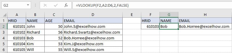
The left table contains employee information like HRID, name, age, and email. HRIDs are unique for employees. A unique HRID is the unique identification of employees. So, when filling employee information (Name in G column and Email in H column) with only HRID supplied, we can use VLOOKUP function to retrieve employee information from corresponding columns of the employee information table. This is a standard usage of VLOOKUP function.
ANALYSIS
In this instance, lookup value is HRID, it is a unique value, it determines which row we can retrieve employee name and email from. And in employee information table, HRID is listed in the first column, name is listed in the second column, email is listed in the fourth column, so we construct the formula below with VLOOKUP function:
Get name =VLOOKUP(F2,A2:D6,2,FALSE)
Get email =VLOOKUP(F2,A2:D6,4,FALSE)
FORMULA
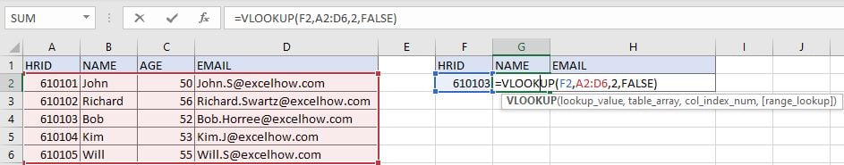
Input formula =VLOOKUP(F2,A2:D6,2,FALSE) into G2, press ENTER, verify that “Bob” is returned properly.
Construction of VLOOKUP function:
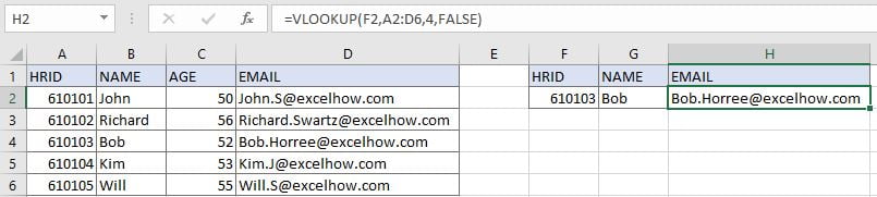
Input formula =VLOOKUP(F2,A2:D6,4,FALSE) into H2, press ENTER, mail address is returned properly.
FUNCTION INTRODUCTION
a. VLOOKUP function looks up the input value from the first column of the given table, and returns the value we want from a particular position (row number depends on the row of lookup value, column number depends on the input argument col_index_num).
Syntax:
=VLOOKUP(lookup_value, table_array, col_index_num,[range_lookup])
For argument “range_lookup”, there are two matching modes “True” and “False”.
- The default mode is “True”, so if this optional argument is omitted, this value is set to “True” automatically.
- If we set “range_lookup” to “True”, VLOOKUP function performs an approximate match.
- If we set “range_lookup” to “False”, VLOOKUP function looks up data restrictively by performing an exact match. If look up value is not found in table, formula returns error “#N/A”.
EXPLANATION
=VLOOKUP(F2,A2:D6,2,FALSE)
lookup_value is HRID “610103” in F2
table_array is A2:D6
col_index_num is 2. Because names are saved in the second column of this table.
range_lookup is set to FALSE. VLOOKUP function performs an EXACT match.
a. In this formula, the look up value is “610103”, VLOOKUP scans this value from the first column of lookup table A2:D6. It continues scanning until it meets the same value. In this case, VLOOKUP function will stop scanning when meeting “610103” in cell A4. As col_index_num is 2, so VLOOKUP function retrieves data at the intersection of row 4 and column 2.
b. We set range_lookup mode to “FALSE”, so VLOOKUP function performs an exact match and this operation can ensure that VLOOKUP keeps scanning till it finds out the same lookup value. If lookup value cannot be found in the first column, an error #N/A will be returned.
Related Functions
- Excel INDEX function
The Excel INDEX function returns a value from a table based on the index (row number and column number)The INDEX function is a build-in function in Microsoft Excel and it is categorized as a Lookup and Reference Function.The syntax of the INDEX function is as below:= INDEX (array, row_num,[column_num])… - Excel VLOOKUP function
The Excel VLOOKUP function lookup a value in the first column of the table and return the value in the same row based on index_num position.The syntax of the VLOOKUP function is as below:= VLOOKUP (lookup_value, table_array, column_index_num,[range_lookup])….