If you are an valid MS Excel user, you have probably come across a situation where you wanted to filter the data in a separate table with complex criteria. You could do this task manually, which is also acceptable while dealing with a few data items.
But if you got a task to filter out multiple items from a table consisting of a lot of data along with specific complex criteria, then doing these kinds of tasks manually would definitely be a stupid decision because this would not only waste your precious time but you would also get tired of it and won’t complete your task on time.
But don’t be worry about it; for getting out of this fix and filtering out multiple data with complex criteria, all you have to do is read this article carefully.
So let’s dive into it.
Table of Contents
General formula:
The formula below would help you filter out multiple data with complex criteria within a few seconds.
As we have altered the following formula according to the example which we would discuss in this article to understand that how this formula works and how to use this formula:
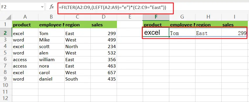
=FILTER(A2:D9,(LEFT(A2:A9)="e")*(C2:C9="East"))
In the formula stated above, we use the filter function and a series of boolean logic expressions.
Let’s See How This Formula Works
In this example, we must create logic that filters data to contain the following conditions: product begins with “e” AND Region is “East“.
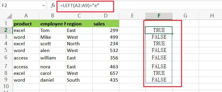
This formula’s filtering logic (the include argument) is built by chaining together two expressions that employ boolean logic on arrays in the data. The first expression used the LEFT function to determine whether product name begins with “e“:
=LEFT(A2:A9)="e" // the product name starts with "e"
As a consequence, an array of TRUE FALSE values looks like this:
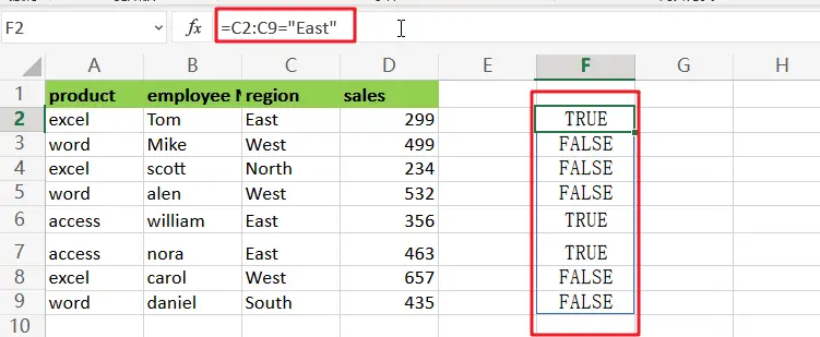
The equal to (=) operator is used in the second equation to see if Region is “East“:
=C2:C9="East" //the region is to the East
As a consequence, another array is created:
=(LEFT(A2:A9)="e")*(C2:C9="East")
The sum of the two arrays is calculated. Because the math process converts TRUE and FALSE values to 1s and 0s.
Because Boolean multiplication corresponds to the logical operator AND, the result is a single array that looks like this:
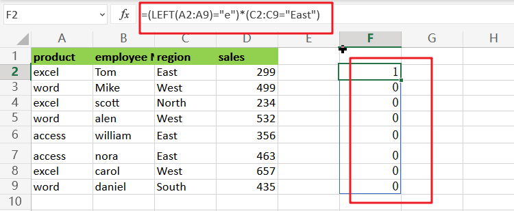
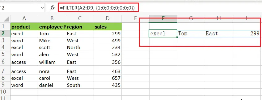
=FILTER(A2:D9, {1;0;0;0;0;0;0;0})
The FILTER function filters the data using this array, returning the one rows that correspond to the 1s in the array.
Advanced Filter allows you to filter data based on numerous criteria
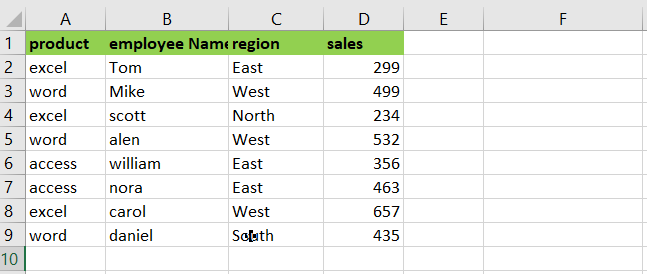
Assume I have the following data list that has to be filtered using several criteria:
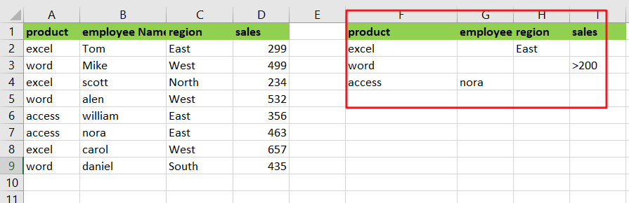
- Product = “excel” and region = “East”,
- The product is “access”, and employee name is “nora”.
- The product is word, and the sales is greater than 200.
And the link is OR among the three criteria.
Please follow the procedures below when using the Advanced Filter function:
Step1: Create your criterion field in an area.See the following screenshot:
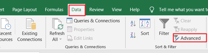
Step2: Select the data range to be filtered and go to Data > Advanced, as shown in the screenshot:
Step3: Finally, in the Advanced Filter dialogue box, click the button next to Criteria range to choose the criteria that I just set, as seen in the screenshot:
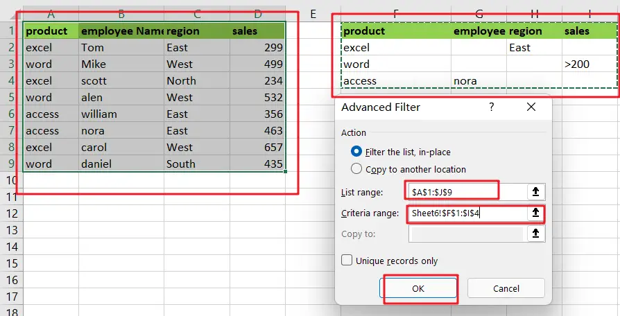
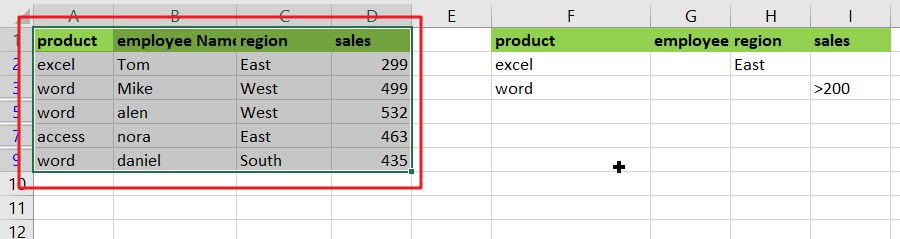
Step4: Then click OK, and the filtered results are displayed; entries that do not meet the criteria are hidden. See the following screenshot:
Related Functions
- Excel Filter function
The FILTER function extracts matched records from a collection of data using one or more logical checks. The include argument specifies logical tests, which might encompass a wide variety of formula conditions.==FILTER(array,include,[if empty])… - Excel LEFT function
The Excel LEFT function returns a substring (a specified number of the characters) from a text string, starting from the leftmost character.The LEFT function is a build-in function in Microsoft Excel and it is categorized as a Text Function.The syntax of the LEFT function is as below:= LEFT(text,[num_chars])…