This post will show you how to use Filter function and in combination with Transpose function to filter data from horizontal and transpose data as vertical in Microsoft Excel.

You can refer to the below general formula based on TRANSPOSE and FILTER function:

=TRANSPOSE(FILTER(range,logic))

You can use the FILTER with TRANSPOSE function to filter data horizontally and show the result in a vertical format. In the below example, the formula in A8 is used:

=TRANSPOSE(FILTER($B$1:$J$3,$B$1:$J$1=2))

1. Filter And Transpose Data From Horizontal To Vertical

This task will filter the horizontal data in range $B$1:$J$3, and display results transposed to a vertical format. We will work with both the data range ($B$1:$J$3) and Class ID range ($B$1:$J$1) in this example.

Filters are one of the most useful functions for organizing your data. You can use them to extract specific pieces or ranges, and they’ll return only what you want! For example, the formula in A8 is:

=TRANSPOSE(FILTER($B$1:$J$3,$B$1:$J$1=2))

The argument includes filter can be used to check for the existence of a file or files. This means it will only return true when the input string matches one or more pattern(s). The syntax looks like this:

$B$1:$J$1=2

The output is an array of 9 TRUE and FALSE values.

{FALSE,TRUE,FALSE,FALSE,TRUE,FALSE,FALSE,TRUE, FALSE }

The input array contains one value per record in the data, and each TRUE corresponds to a “2” Class ID column. This returning value is then used by FILTER as an argument for its filtering:

FILTER($B$1:$L$3,{FALSE,TRUE,FALSE,FALSE,TRUE,FALSE,FALSE,TRUE, FALSE })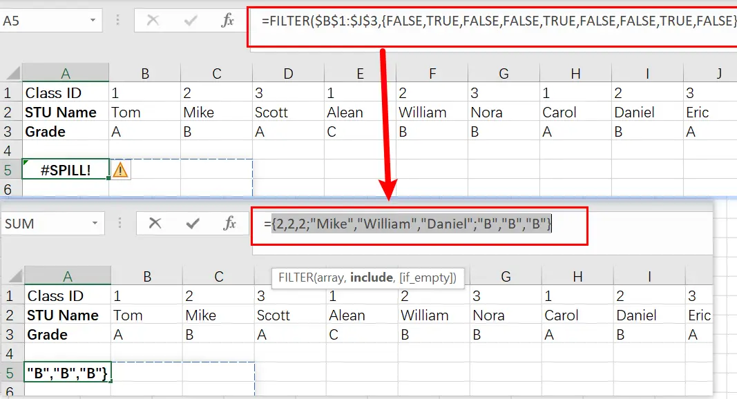

By only passing through columns that correspond with TRUE, the result is a set of data for those three people in  Class 2. FILTER gives us back this original format but displays it vertically instead! The TRANSPOSE function was included so we can see they’re displayed properly.

=TRANSPOSE(FILTER($B$1:$J$3,$B$1:$J$1=2))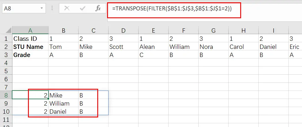

By using the TRANSPOSE function, we can transform our data into a vertical array. This means that when there is a variation in any of cells B1 through J3 (or their values), all filter results will be updated automatically!

2. Video: Filter And Transpose Data From Horizontal To Vertical

This video tutorial will show you how to use Filter function in combination with Transpose function to filter data from horizontal and transpose data as vertical in Microsoft Excel 365.

3. Related Functions

• Excel Filter function
  The Excel  FILTER function extracts matched records from a collection of data using one or more logical checks. The include argument specifies logical tests, which might encompass a wide variety of formula conditions.==FILTER(array,include,[if empty])…
• Excel TRANSPOSE function
  Excel TRANSPOSE formula allows you to rotate (swap) values from rows to columns and vice versa in Excel.The Excel TRANSPOSE Function syntax:=TRANSLATE (range) …