Excel TRANSPOSE formula allows you to rotate (swap) values from rows to columns and vice versa in Excel. Its goal, as a component of the Excel lookup and reference functions, is to arrange data in the appropriate manner. To run the formula, pick the precise size of the transposed range and hit the CSE key (“Control+Shift+Enter“).
Table of Contents
Description
The TRANSPOSE function in Microsoft Excel returns a transposed range of cells. For instance, if a vertical range is specified as a parameter, a horizontal range of cells is returned. Alternatively, if a horizontal range of cells is specified as a parameter, a vertical range of cells is returned.
Excel TRANSPOSE formula is an Excel built-in function that is classified as a Lookup/Reference Function. It may be used in Excel as a worksheet function (WS). The TRANSPOSE function is a worksheet function that may be used as part of a formula in a worksheet cell.
Syntax
The Excel TRANSPOSE Function in Microsoft Excel has the following syntax:
=TRANSLATE (range)
Arguments or Parameters:
range – The range of cells to transpose.
Returns
TRANSPOSE returns a range of cells that have been transposed.
Note:
The TRANSPOSE function requires an array as the range value. Enter a value and then press Ctrl+Shift+Enter to create an array. This will enclose the formula in brackets, indicating that it is an array.
Applicable To
Notes on use:
- The TRANSPOSE function transforms a vertical range of cells to a horizontal range of cells, or vice versa. TRANSPOSE, in other terms, “flips” the orientation of a specified range or array:
- TRANSPOSE translates a vertical range to a horizontal range when provided one.
- TRANSPOSE transforms a horizontal range to a vertical range when provided one.
- When an array is transposed, the first row becomes the new array’s first column, the second row becomes the new array’s second column, the third row becomes the new array’s third column, and so on.
- TRANSPOSE is a function that works with both ranges and arrays. Ranges that have been transposed are dynamic. If the data in the source range changes, TRANSPOSE updates the data in the target range instantly.
Excel TRANSPOSE Function
The TRANSPOSE Excel function, as the name implies, may be used to transpose data in Excel.
The syntax is as follows:
=TRANSPOSE(array)
The array denotes a range of cells to be transposed in this case.
Take the following basic steps:
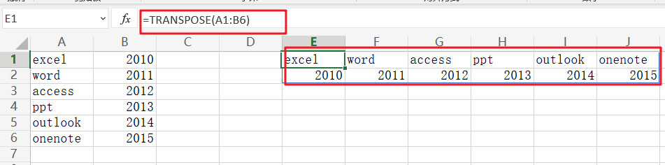
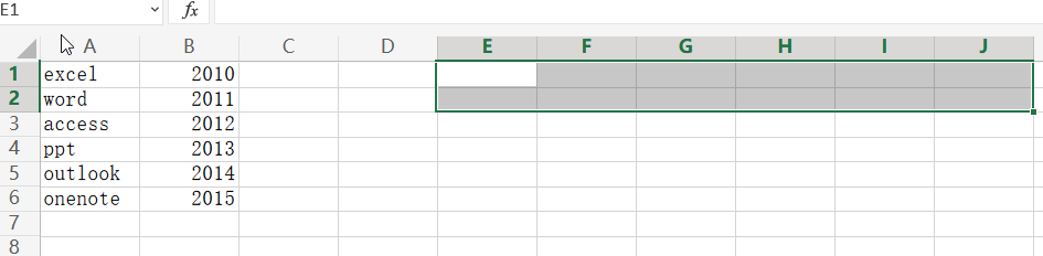
Step1: Choose the range of cells in which you wish the output data to be transposed.
Step2: TRANSPOSE is an array formula; hence, the precise amount of cells must be specified.
Step3: If the range of your table is 6×2, i.e., 6 rows and 2 columns, you must pick a 2×6 range for the transposed data, i.e., 2rows and 6 columns.
Step4: Insert the formula =TRANSPOSE (A1:F5)
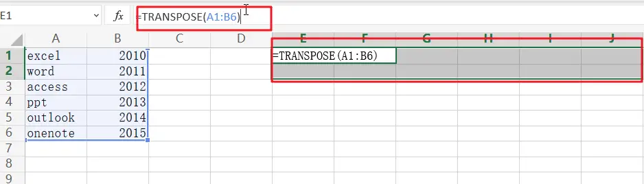
Step5: Avoid pressing Enter! Ctrl+Shift+Enter is required to perform array formula.
Step6: It’s worth noting that transpose is an array formula. An array formula must be input by hitting the Ctrl+Shift+Enter key combination, which causes the formula bar to insert a set of braces around the formula.
Step7: This instructs Excel to print an array of data rather than a single cell.
Step8: Transposition of the data is now complete.