You might have been through this kind of situation where you need to filter out the horizontal data from the list having few columns. I am also pretty sure about it that you might have chosen to do it manually, which is also a great choice when you have only a few values in a list, and you want to filter out the top n values.
However, if you are dealing with numerous columns in the list and want to filter out the horizontal data, then executing these jobs manually would be a stupid move since there is a 90% probability that you will become weary of it and will be unable to accomplish your assignment on time.
But don’t worry about it, since after attentively reading this post, filtering out horizontal data from a list with many values will be a piece of cake for you.
So let’s go into the article and solve this problem.
Table of Contents
General Formula
The Following formula would help you Filter the horizontal data in MS Excel:
=FILTER(data_range,criteria)
Explanation of Syntax
Before we go into the formula for getting the job done quickly, we need to understand each syntax to comprehend how each syntax helps filter out the horizontal data in MS Excel.
Filter: This function contributes to narrowing down or filtering out a range of data on the user-defined criteria.data_range: In your worksheet, it represents the input ranges.Comma symbol (,): In Excel, this comma symbol acts as a separator that helps to separate a list of values.criteria: the criteria on which you want to collect or filter the data.Parenthesis(): The core purpose of this Parenthesis symbol is to group the elements and separate them from the rest of the elements.
Let’s See How This Formula Works
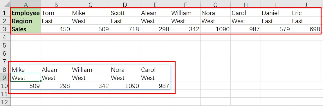
For understanding easily that how this formula works and how to use this formula, Suppose that you got a task in which three horizontal rows have multiple columns, each horizontal row have different types of data; now you want to filter out data from these horizontal rows on a certain logic or criteria.
As to filter the horizontal data on a certain logic, we would write the formula according to the given list like:
=FILTER(data_range,region="West")
Here in this formula, the named ranges are data_range (B1:J3) and region (B2:J2)
Please remember that FILTER is a new dynamic array function in Excel 365. There are equivalents in other versions of Excel, but they are more Sophisticated.
The primary goal is to filter this horizontal data to extract only columns (records) with the region “West“.
The FILTER function can extract data that is arranged vertically (in rows) or horizontally (in columns). The matching data will be returned in the same orientation by the FILTER function.
There is no special setup required. The formula in A8 in the example shown is:
=FILTER(data_range,region="West")
The included argument for FILTER is a logical expression that works from the inside out:
=region="West"/ look for the word "West "
When the logical expression is evaluated, it yields an array of ten TRUE and FALSE values:
{FALSE,TRUE,FALSE,TRUE,TRUE,TRUE,TRUE,FALSE,FALSE}
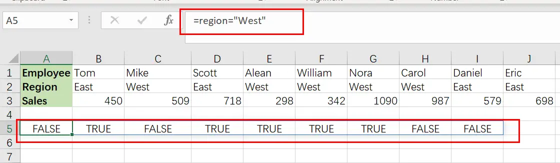
It’s worth noting that the commas (,) in this array indicate columns. Rows would be indicated by semicolons (;).
The array has one value for each column of data, and each TRUE corresponds to a column with the region “ West” .
This array is passed straight to FILTER as the included parameter, and it conducts the filtering of the data:
=FILTER(data_range,{ FALSE,TRUE,FALSE,TRUE,TRUE,TRUE,TRUE,FALSE,FALSE })
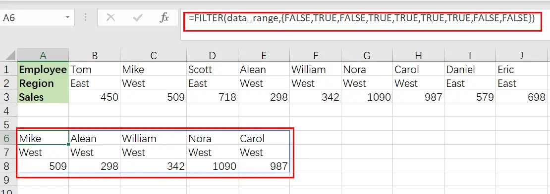
Because the filter only accepts data corresponding to TRUE values, FILTER delivers the 5 columns where the region is “ West“.
This data is returned by FILTER in its original horizontal layout.
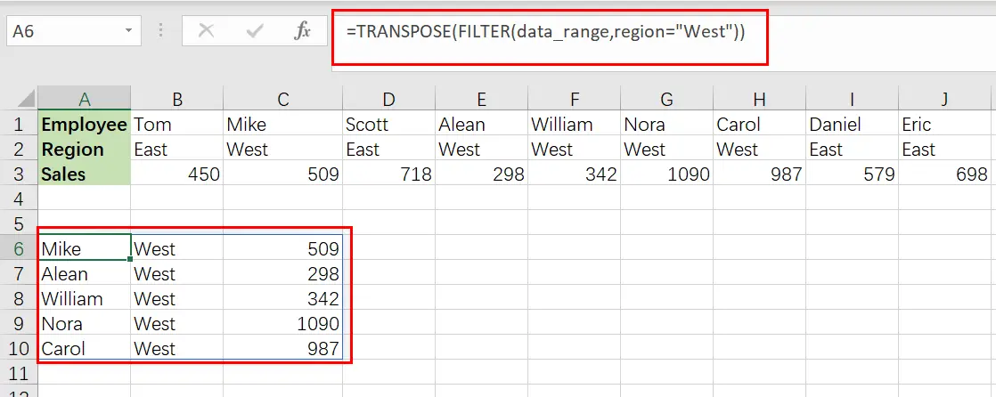
Transpose Filter Results
If you want to transpose the filter results into a vertical format, you can use the TRANSPOSE function around the FILTER function like follows:
=TRANSPOSE(FILTER(data_range,region="West"))
The result is as follows:
Filter Data by Another Column
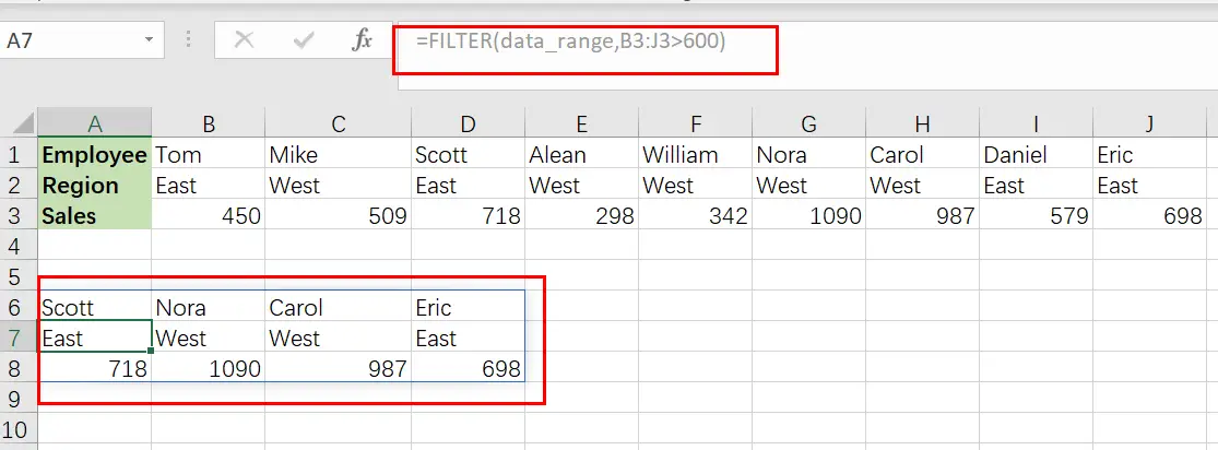
The same fundamental method may be used to filter data in a variety of ways. For instance, if you want to filter out data to show only columns with sales greater than 600, just use the following formula based on the FILTER function:
=FILTER(data_range,B3:J3<600)
Related Functions
- Excel Filter function
The Excel FILTER function extracts matched records from a collection of data using one or more logical checks. The include argument specifies logical tests, which might encompass a wide variety of formula conditions.==FILTER(array,include,[if empty])… - Excel TRANSPOSE function
Excel TRANSPOSE formula allows you to rotate (swap) values from rows to columns and vice versa in Excel.The Excel TRANSPOSE Function syntax:=TRANSLATE (range) …