Assume that you’re in a situation where you need to filter every nth row from a list having a few values. I’m pretty sure you’d choose to do it manually, which is also a great choice when you only have a few values in a list and want to filter out every nth row.
However, if you are dealing with several values in the list and want to filter out the nth row, then executing these jobs manually would be a stupid move since there is a 90% probability that you will become tired of it and will be unable to accomplish your assignment on time.
But don’t worry, after carefully reading this post, filtering off every nth row from a list with multiple values will be a piece of cake for you.

So let’s go into the article and get you out of this bind.
Table of Contents
The formula in General
In MS Excel, use the following formula to filter every nth row:
=FILTER(total_data,MOD(SEQUENCE(ROWS(total_data)),n)=0)
Explanations of Syntax
Before we get into the formula for getting the job done quickly, we need to grasp each syntax to see how each syntax helps filter out every nth row in MS Excel.
-
Filter: This tool helps narrow down or filter out a range of data based on user-defined criteria. -
Comma symbol (,): In Excel, this comma symbol serves as a separator, aiding in separating a list of values. total_data: is nothing more than representing each column in the list.Parenthesis(): The primary function of this Parenthesis symbol is to group and separate elements.ROWS: This refers to the nth row you want to filter out.MOD(): The MOD function accepts two real number operands as inputs and returns the remainder of dividing the integer component of the first parameter (the dividend) by the integer part of the second argument (the divisor)SEQUENCE(): The SEQUENCE function in Excel lets you create a sequence of consecutive numbers in an array, such as 1, 2, 3, 4.
Let’s See How This Formula Works
For example, suppose you have a task in which there is a table with candidates from two regions (i.e., West and East ) and which are assigned to a particular sales number; now you want to filter out every second row, which is the sequence which we would write in the formula; now let’s analyze how to write the formula and how this formula would do it.
To filter every second row, we would use the following formula based on the supplied list:
=FILTER(A2:C10,MOD(SEQUENCE(ROWS(A2:C10)),2)=0)
To filter and extract every nth row, use a formula that combines the FILTER function with MOD, ROW, and SEQUENCE. Where data refers to the designated range A2:C10. With n hardcoded as 2, the FILTER function retrieves every third row in the data.
The FILTER function filters and extracts data based on logical criteria. This example aims to extract every second record from the supplied data, although there is no row number information in the data range A2:C10.
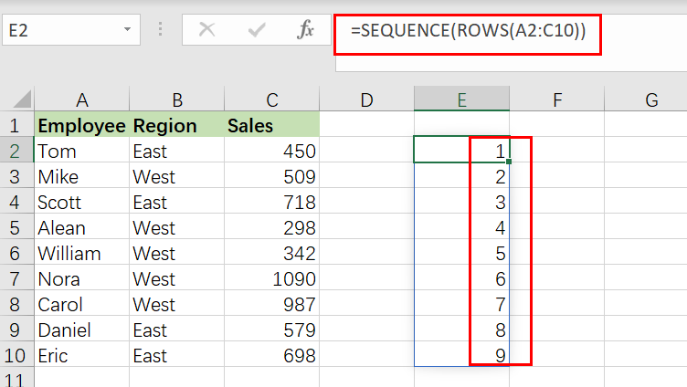
The first stage, working from the inside out, is establishing a row number set. This is accomplished using the SEQUENCE function as follows:
=SEQUENCE(ROWS(A2:C10))
The ROW function returns the number of rows in the specified range of data. SEQUENCE provides an array of 9 integers in sequence based on the number of rows:
{1;2;3;4;5;6;7;8;9}
This array is sent straight to the MOD function as the number parameter, with the divisor hardcoded as 2. MOD is configured to check if row numbers are divisible by 2 with a remainder of zero.
=MOD(SEQUENCE(ROWS(A2:C10)),2)=0 /// is it divisible by 2?
MOD produces an array of TRUE and FALSE values, as shown below:
{FALSE;TRUE;FALSE;TRUE;FALSE;TRUE;FALSE;TRUE;FALSE}
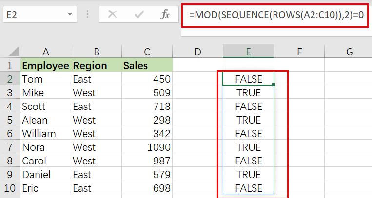
Take note that TRUE values correlate to every second row in the data range A2:C10. This array is passed straight to the FILTER function as the include parameter. As a final result, FILTER returns every second row of data.
Related Functions
- Excel Filter function
The Excel FILTER function extracts matched records from a collection of data using one or more logical checks. The include argument specifies logical tests, which might encompass a wide variety of formula conditions.==FILTER(array,include,[if empty])… - Excel MOD function
the Excel MOD function returns the remainder of two numbers after division. So you can use the MOD function to get the remainder after a number is divided by a divisor in Excel. The syntax of the MOD function is as below:=MOD (number, divisor)…. - Excel ROWS function
The Excel ROWS function returns the number of rows in a cell reference.The syntax of the ROWS function is as below:= ROWS(array)…