Just assume that you have two lists containing values/words in the few cells, and you want to extract the same or common values/words from the two lists into another separate list; then you might think that it’s not a big deal; because you would prefer to manually extract the same or common values/words from the two lists into another separate list without any need of the formula.
Then congratulations because you are thinking right, but let me include that it would be a big deal to extract the same or common values/words from the two lists including multiple cells into another separate list and doing it manually would be a foolish attempt, because there are 90% chances that you would 100% get tired of it and would never complete your work on time.
But don’t be worry about it because after carefully reading this article, extracting the same or common values/words from the two lists into another separate list would become a piece of cake for you.
So let’s dive into the article to take you out of this fix.
Table of Contents
General Formula
The Following formula would help you compare and extract the same or common values/words from the two lists into another separate list.
=FILTER(Table1,COUNTIF(Table2, Table1))
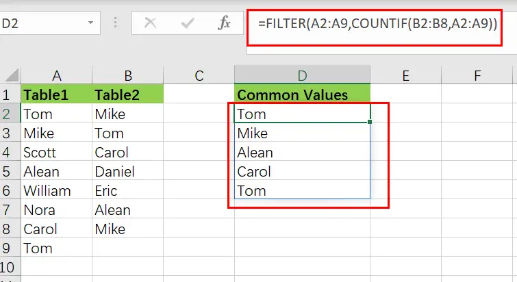
This Formula is based on the FILTER and COUNTIF function, where the Table1 (A2:A7) and Table2 (B2:B7) are the named ranges, the table in the range D2:D7 is the common list containing the common elements or values by comparing both Table1 and Table2.
Syntax Explanations:
Before going into the explanation of the formula for getting the work done efficiently, we must understand each syntax which would make it easy for you that how each syntax contributes to executing the same or common values/words from the two lists into another separate list:
Filter: This function contributes to narrowing down or filtering out a range of data on the user-defined criteria.COUNTIF: It is a statistical function that contributes to counting the number of cells to meet specific criteriaList: In this formula, the list represents the two lists present in the excel worksheet to execute the common valuesComma symbol(,): In Excel, this comma symbol acts as a separator that helps to separate a list of values.Parenthesis(): The core purpose of this Parenthesis symbol is to group the elements and to separate them from the rest of the elements.
Let’s See How This Formula Works:
The FILTER function takes an array of values as input and an “include” parameter to filter the array based on a logical expression or value.
The array is provided in this example as the named range “Table1“, which contains all values in the range A2:A7. The COUNTIF function, which is nested inside FILTER, provides the included argument:
=FILTER(Table1,COUNTIF(Table2, Table1))
COUNTIF is set up with Table1 as criteria and Table2 as the range. Because if the eight criteria values are given to the COUNTIF, then as an array, it would also return eleven results like the following:
{1;1;0;1;0;1;0;1;0;1;1}
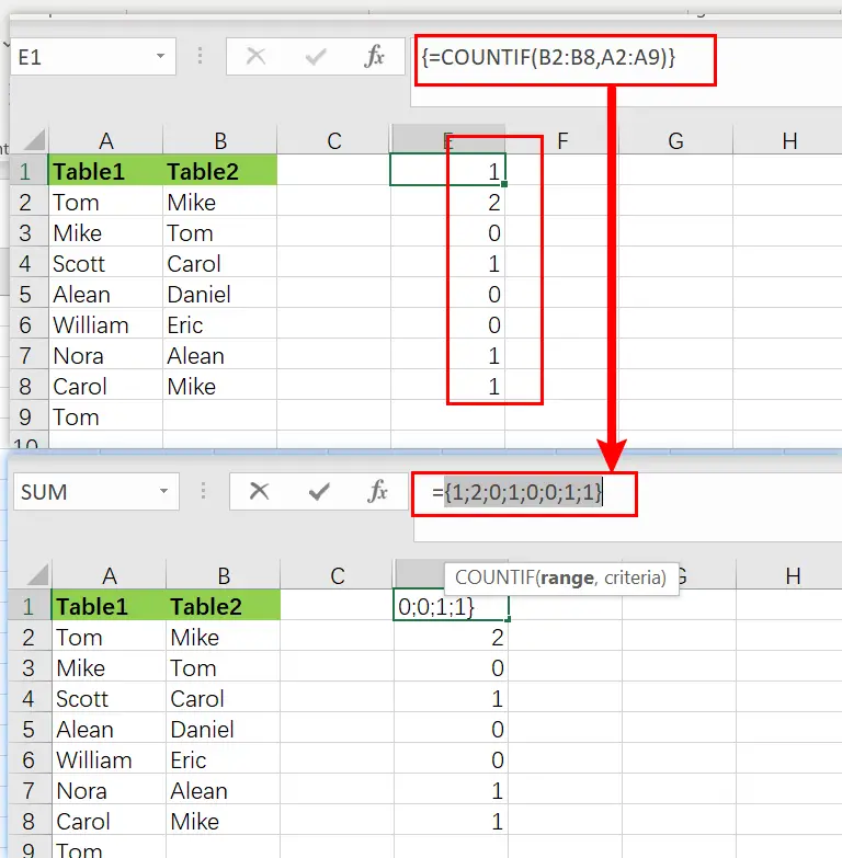
Keep it into your notice that the 1’s correspond to the Table2 items, which also appear in the Table1.
As with the aid of “include” argument this array is delivered to the FILTER function directly:
=FILTER(Table1,{1;1;0;1;0;1;0;1;0;1;1})
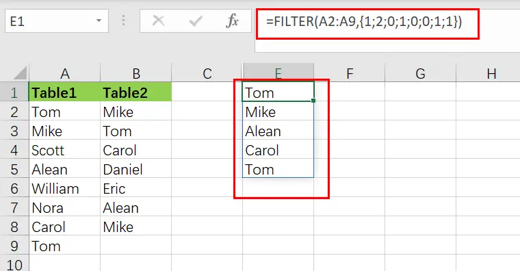
Using the values provided by COUNTIF, the FILTER function efficiently filters the Table1. The values except zero are preserved, and the values associated with zero are removed.
The list spread into the range D2:D7 is the final result consisting of an array of values common in both Table1and Table2.
More Examples
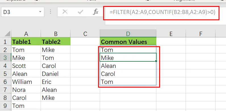
The raw results from COUNTIF are used as the filter in the above algorithm. This works because Excel considers any non-zero number to be TRUE and any zero value to be FALSE. If COUNTIF returns a count larger than one, the filter will continue to function normally.
You can use “>0” to force TRUE and FALSE results explicitly, like as follows:
=FILTER(Table1,COUNTIF(Table2,Table1)>0)
Remove duplicates From Common Values
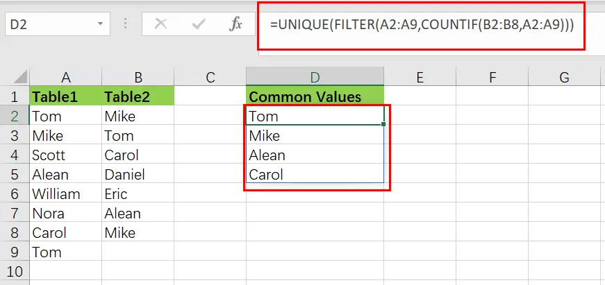
Nest the formula inside the UNIQUE function to remove the duplicates, just like as follows:
=UNIQUE(FILTER(Table1,COUNTIF(Table2,Table1)))
Sort Common Values
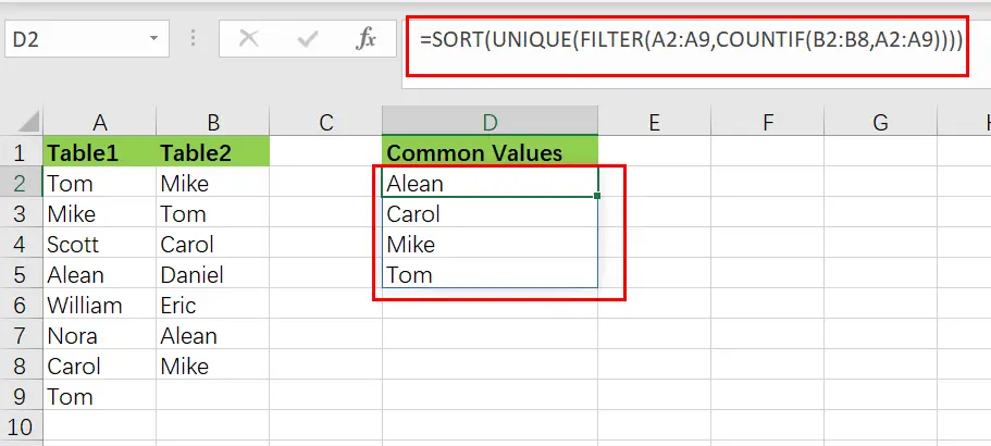
Just nest the formula in the SORT function to sort results:
=SORT(UNIQUE(FILTER(Table1,COUNTIF(Table2,Table1))))
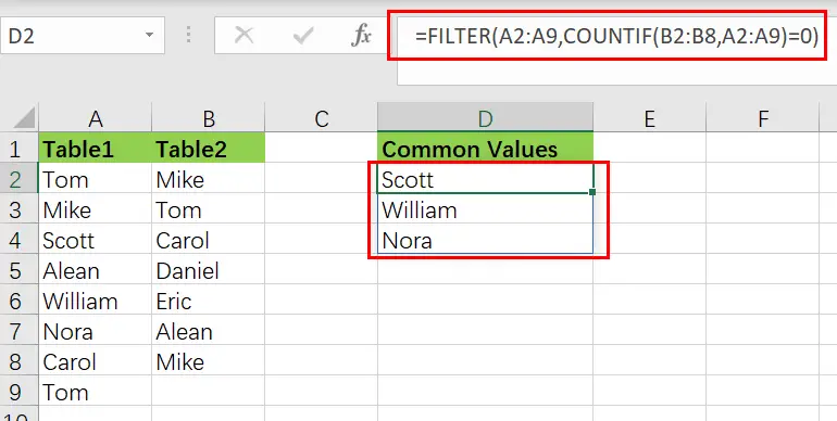
Extract values missing from Table2
You can reverse the logic for getting the output values in Table1 missing from Table2, like in the follows:
=FILTER(Table1,COUNTIF(Table2,Table1)=0)
Related Functions
- Excel COUNTIF function
The Excel COUNTIF function will count the number of cells in a range that meet a given criteria. This function can be used to count the different kinds of cells with number, date, text values, blank, non-blanks, or containing specific characters.etc.= COUNTIF (range, criteria)… - Excel Filter function
The FILTER function extracts matched records from a collection of data using one or more logical checks. The include argument specifies logical tests, which might encompass a wide variety of formula conditions.==FILTER(array,include,[if empty])… - Excel Sort function
The SORT function in Excel sorts the contents of an array or range alphabetically or numerically by columns or rows.The syntax:=SORT(array, [sort index],) … - Excel UNIQUE function
The guide demonstrates how to use the UNIQUE function and dynamic arrays in Excel to create unique values.The syntax:=UNIQUE(array, [by col], [once exactly]) …