This post will guide you how to create pie of pie or bar of pie charts in Excel. The pie of pie charts is used to represent separate tiny slices from the main pie chart and show them in additional pie charts in your current worksheet.

Create Pie of Pie

---

To create a pie of pie chart in your worksheet, you need to do the following steps:

#1 select the range of cells as source data to create chart

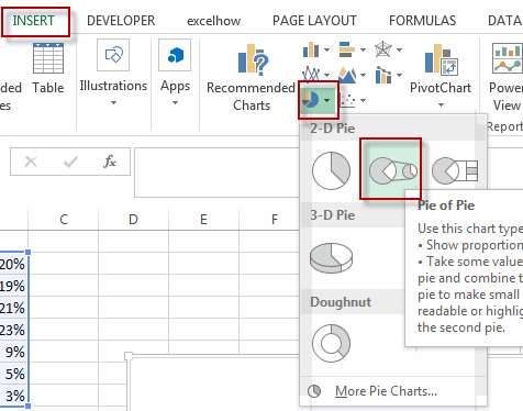
#2 go to INSERT tab, click Insert pie command under Charts group. And select Pie of Pie from the 2-D Pie section in the drop-down menu list.

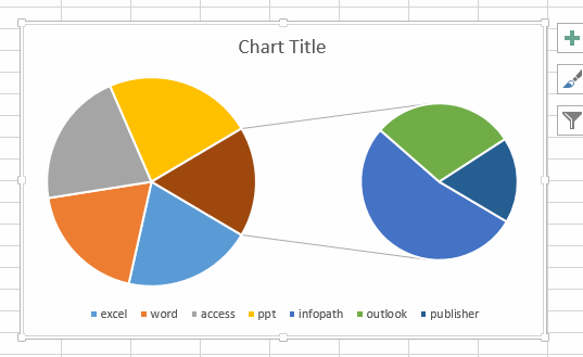
#3 the Pie of Pie chart has been created.

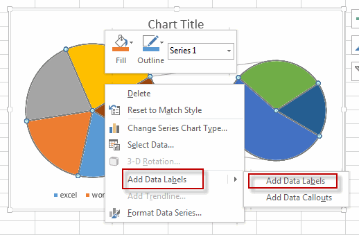
#4 click on the data series, and right click on it, select Add Data Labels from the popup menu list.

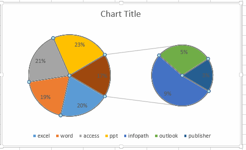
#5 the data labels are added into the all data series.

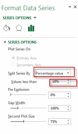
#6 right click on the selected data series, and select Format Data Series from the popup menu list. The Format Data Series pane will appear.

#7 select Percentage value in the Split Series By list box. And type one percentage value (such as: 10% ) in the text box of the Values less than.

#8 close the Format Data Series pane.

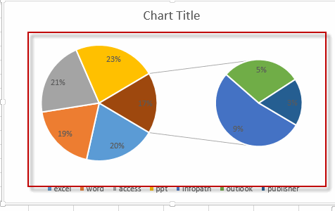
#9 let’s see the result.

Create Bar of Pie chart

---

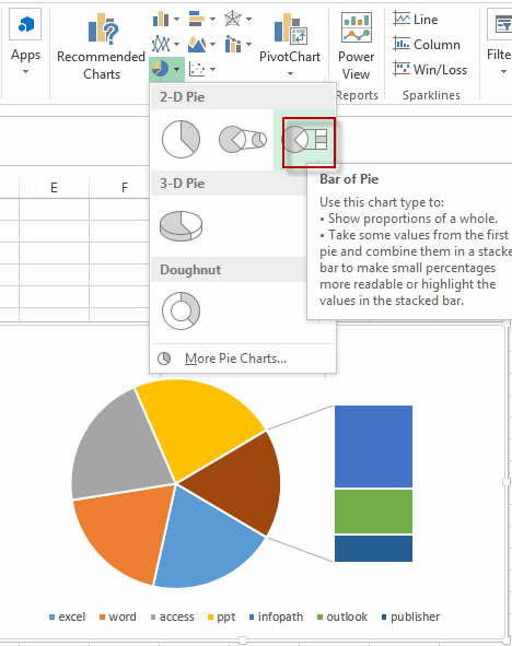
If you want to create a Bar of Pie chart in your worksheet based on the source data, you just need to go to INSERT tab, click Insert pie command under Charts group. And select Pie of Bar from the 2-D Pie section in the drop-down menu list.

The repeat the above steps from 3-9.