Assume that you got a task to convert the full state’s name into the abbreviations in MS Excel, and for doing this task, you might choose to do it manually, which is an acceptable way only if you don’t have any other way to do it!
But fortunately, there is a way to convert a state’s name into abbreviations, and after reading this article carefully, you would get to know about that way by which you can do this task in a few seconds.
So let’s get straight into it.

Table of Contents
1. Convert State Names To Abbreviations
a. General Formula
The Formula to convert state names to the abbreviations in a matter of seconds is mentioned as follows:
=VLOOKUP(States_Name,states_Data,2,0)b. Explanation of Syntax
Before getting knowledge about how to use this Formula to get the work done, we first need to understand how each syntax of the Formula contributes to making this Formula worthful:
VLOOKUP: The VLOOKUP function retrieves data from a range or table row by row.Parenthesis(): The primary function of this symbol is to group the elements.
Let’s See How This Formula Works
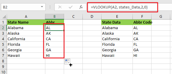
A simple formula based on VLOOKUP may be used to convert complete state names to their two-letter abbreviation. The Formula in B2 in the example is:
=VLOOKUP(A2, states_Data,2,0)
Where “ states_Data ” refers to the designated E2:F7 range:
This means that this method is based on a database with columns for the full state name and the 2-letter abbreviation. Because we’re using VLOOKUP, we need the whole name in the first column. The table has been dubbed “states_Data” for clarity’s sake.
VLOOKUP is set to retrieve the lookup value from column A. The table array represents the designated range “ states_Data,” The column index is 2 (to extract the abbreviation from the second column). The final option, range lookup, has been set to zero (FALSE).
VLOOKUP finds the matching entry in the “states_Data” database and returns the 2-letter abbreviation.
2. Convert Abbreviations to State Names (Lookup In Reverse)
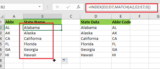
What if you have an abbreviation of the states and want to search up the complete state name in the sample lookup table? You’ll need to use INDEX and MATCH instead in such a situation. With a lookup value in A2, this Formula will yield the whole state name as shown in the lookup table:
=INDEX(D2:D7,MATCH(A2,E2:E7,0))
You may use this version to convert a 2-letter abbreviation to a complete state name if you wish to utilize the same-named range “ states_Data.”
=INDEX(INDEX(states_Data,0,1),MATCH(A1,INDEX(states_Data,0,2),0))
By specifying a row number of zero, we may utilize INDEX to return whole columns. This is an interesting and helpful aspect of the INDEX function: if you specify zero for the row, you receive complete column.
You may convert abbreviations to complete state names using the INDEX and MATCH methods. The INDEX and MATCH functions can help you out to retrieve the complete state names depending on the abbreviations.
3. Video: Convert State Names To Abbreviations
This video will show you how to convert state names to abbreviations in Excel using a formula.
4. Related Functions
- Excel VLOOKUP function
The Excel VLOOKUP function lookup a value in the first column of the table and return the value in the same row based on index_num position.The syntax of the VLOOKUP function is as below:= VLOOKUP (lookup_value, table_array, column_index_num,[range_lookup])…. - Excel INDEX function
The Excel INDEX function returns a value from a table based on the index (row number and column number)The INDEX function is a build-in function in Microsoft Excel and it is categorized as a Lookup and Reference Function.The syntax of the INDEX function is as below:= INDEX (array, row_num,[column_num])… - Excel MATCH function
The Excel MATCH function search a value in an array and returns the position of that item.The MATCH function is a build-in function in Microsoft Excel and it is categorized as a Lookup and Reference Function.The syntax of the MATCH function is as below:= MATCH (lookup_value, lookup_array, [match_type])….