In Microsoft Excel Spreadsheet or google sheets, conditional formatting is used to highlight any cell based on a predefined condition and the value of those cells. In the previous article, we described how to format a specific column or cell range based on another cell value in Excel or google sheets.

In Excel or Google sheets, it is relatively easy to apply conditional formatting based on the current value of a cell. However, suppose you run into a problem where you have to highlight or format a column based on the value of another column. You can use conditional formatting based on another column to solve such problems.

This article will describe in detail how to format another column based on another column’s value in a Microsoft Excel spreadsheet or Google Sheets.

EXAMPLE

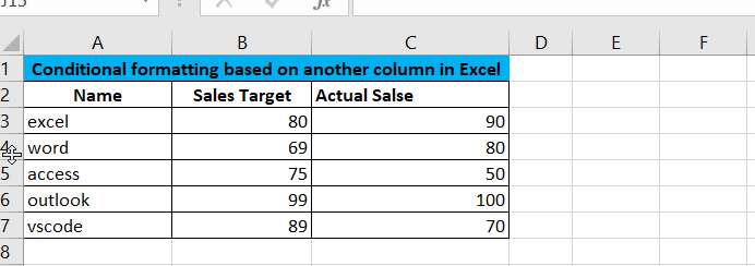
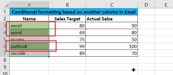
The following is an example that can be used to demonstrate the application of conditional formatting functionality in an instance. Suppose you have a product sales table with a sales target and an actual sales value for each month, now let’s use conditional formatting to find the product names whose actual sales are higher than the sales target. Below is a screenshot of our product sales table.

Below we will introduce how to customize conditional formatting rules by formulas to format cells in one column based on the value of another column in Microsoft Excel Spreadsheet and Google sheets respectively.

Highlight Cells Based on Another Cell in Excel

If you want to highlight a column based on the value of another column, then you can create custom conditional rules in Conditional Formatting. The specific steps are as follows.

Step1: Select the column to which you want to apply the custom condition rule, for example: A3:A7.

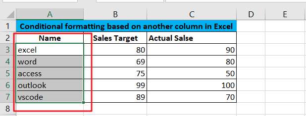
If you want to apply conditional formatting, you must first select the cells. If you want to highlight the entire row after applying conditional formatting, you need to select all the data sets. But to highlight the cells of a column, you only need to select the cells of that column. If you want to highlight an entire row or column, then you need to select that column or row.

In the example in this article, you need to select the name column first, i.e. A3:A7

Step2: You need to open the Conditional Formatting panel and select the appropriate formatting rule as needed. In Ribbon, select HOME->Conditional Formatting -> New Rule, New Formatting Rule dialog will open.

Note: To apply conditional formatting to a column based on another column, we need to select the New Rule menu.

Step3:  From the list of rule types below, we can see the type of rule we need, that is, we want to determine the cells to be formatted by a formula. We need to select: Use a formula to determine which cells to format.

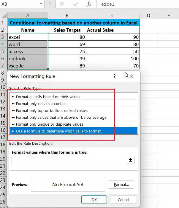
Note: As you can see from the image above, the New Formatting Rule dialog box has a number of rule types, such as: Format all cells based on their values, Format only cells that contain, Format only top or bottom ranked values, Format only values that are above or below average , Format only unique or duplicate values and Use a formula to determine which cells to format.

When the formatting formula returns a True value, the cell will be applied to the corresponding format, and if the formula returns False, then the formula will not be applied.

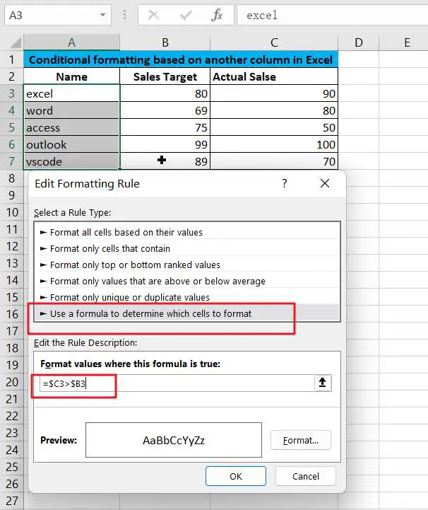
Step4: When you select the “Use a formula to determine which cells to format” rule type, the box named “Format values where this formula is true ” will appear below the “Select a Rule Type” box. Enter the following formula in the Format values where this formula is true text box:

=$C3>$B3

Note: The formula above compares the value of column C with the value of column B in the same row. If the value of column C is greater than the value of column B in the same row, then the cells in column A will be formatted.

Step5: Click the “Format” button to select a format for the cells that match the criteria. After setting your preferred formatting style, click the OK button.

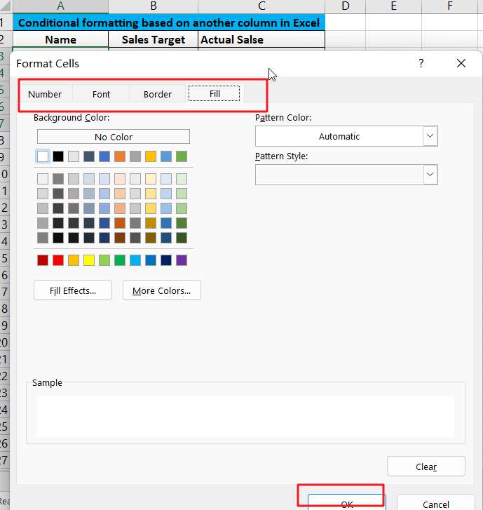
Step6: You will see your selected formatting style in the Preview box of the New Formatting Rule window. After clicking OK, the selected formatting will be applied to the cells that meet the conditions.

Highlight Cells Based on Another Column in Google Sheets

The following is a conditional formatting function to highlight the cells in the name column that match the condition based on the column value in the Google Sheet spreadsheet. The steps are as follows.
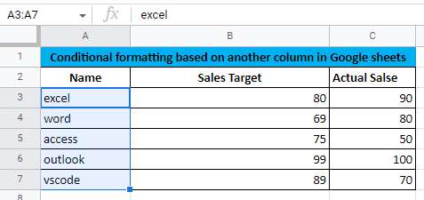
Step1: In this case, select the product name column (excluding the title) A3:A7 and it will be highlighted in blue.

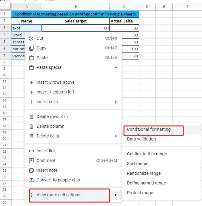
Step2: Click the “Format” menu and then click the “Conditional Formatting” menu.

Or right-click on the selected column -> select “View more cell actions” -> “ Conditional formatting “, the Conditional formatting rules dialog box will pop up.

Step3: Next we can select the desired format for the range or column. Select Single color Tab

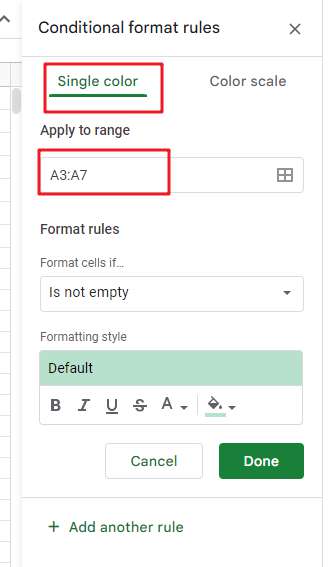
Note: We can also select the range of cells by manually selecting them in the Conditional Formatting Rules window. For example, if we choose to conditionally format the first 100 cells of column A, we can specify the range to apply to as “A3: A103”.

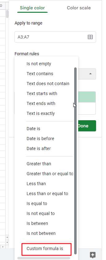
Step4: Select “Custom formula is” from the “Format Cells if” drop-down list

Step5: In the Formula text box, enter the following formula.

=$C3>$B3

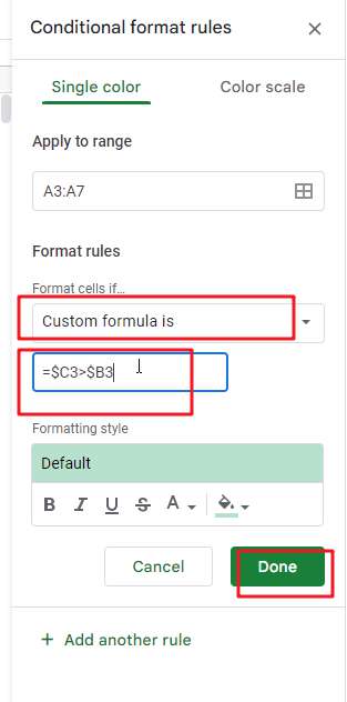
The formula here is the actual sales value corresponding to the product name cell is greater than the sales target value. The formula becomes “=$C3>$B3” because the actual sales value is in column C with the first cell row number of 3, and the sales target value is in column B with the first cell row number of 3.

The formula uses the greater than operator (>) to evaluate each cell in C3:C7 to the corresponding cell in B3:B7. When the formula returns “true”, the rule is triggered and the highlighting format is applied.

Step6: Select a style from the “Formatting style” drop-down list

Step7: Click the “Done” button

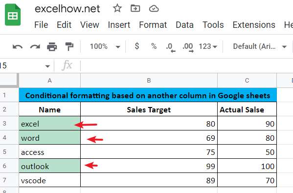
As you can see from the image above, you will see that the cell containing the name will be conditionally highlighted based on the value of another column.

Conditional Formatting Based On Another Column FAQ

How do you conditional formatting in Excel based on another column text?

1. Select the cell to which you want to apply conditional formatting. Click the first cell in the range, then drag it to the last cell.
2. Click Home > Conditional Formatting > Highlight Cell Rules > Included Text…
3. Select the color formatting for the text, and then click OK.

How do you conditional format if one column is greater than another?

1. Do one of the following to open the dialog box. choose Data > Conditional Formatting > Highlight Cell > Greater Than.

Can you use conditional formatting to compare two columns?

1. If you want to compare two columns and highlight the matching data, you can use the duplicate function in conditional formatting.

How do you conditional format a range based on another range?

1. Select all cells in the worksheet that you want to highlight and apply formatting rules to.
2. Click Conditional Formatting.
3. Select the Highlight Cells rule, and then select the rule that applies to your needs…
4. Fill out the Less Than dialog box and select a formatting style from the drop-down menu.

Video: Conditional Formatting Based On Another Column in Excel/google sheets

Conclusion

This article provides you with a base method for conditional formatting of an entire column based on another column in Excel and Google sheets. Therefore, if you follow the steps described in this article, you will be able to apply conditional formatting to columns based on the conditions of other columns.

Sample files

Below are sample files in Microsoft Excel and google sheets that you can download for reference if you wish.