In Microsoft Excel Spreadsheet or google sheets, when you want to format a specified cell or cell range based on the value of a different cell, for example, formatting the first row based on the value of a cell in a single column, you can use the conditional formatting function to create formatting formulas.

This article will talk in detail about how to format a cell range based on the value of another cell in a Microsoft Excel spreadsheet or Google Sheets.

EXAMPLE

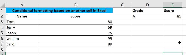
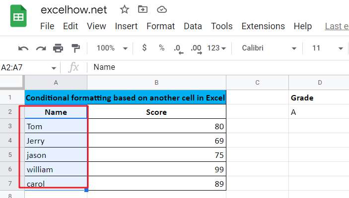
The following is an example that can be used to demonstrate how to apply conditional formatting functions in an instance. Suppose you have a table of student scores and you need to determine the names of students with scores greater than 85. Below is a screenshot of our sample student score table.

There are several ways to find and print out the names of students with grades greater than 85 in Excel or Google Sheet. You can use the IF function to do a score comparison and then print out the cell values that meet the criteria. Another way is to use the conditional formatting function to quickly highlight the names that meet the criteria.

Conditional format function introduction

You can easily highlight specific columns with the conditional formatting function, because the cells to be formatted are highlighted if they are the same as the cells to be evaluated or if they match a condition. That is, we can format the cell state of the column in which the same type of value is located based on the value of a cell as a condition.

To accomplish the above and simply highlight the status of the Score column, the following steps can be performed.

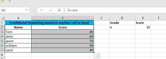
STEP 1: Select the Score column

STEP2: Click HOME Tab, in the Styles group, click Conditional Formatting command, click Highlight Cells Rules menu, and then click the cell rules in the secondary menu, such as: Greater Than, Less Than, Between, Equal To ,etc.

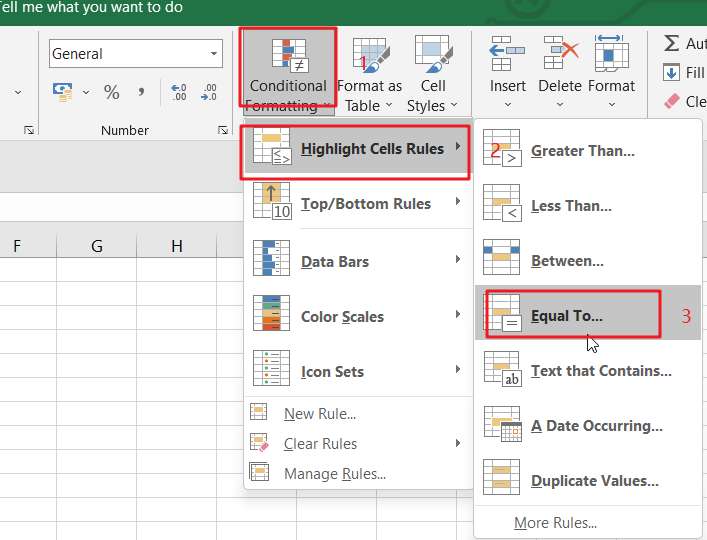
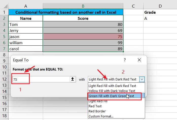
In this example, we select the Equal To cell rule. Then the Equal To dialog box will pop up.

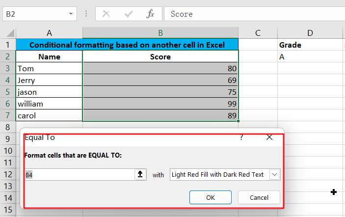
Step3: We can enter 75 in the Format cells that are EQUAL TO: text box, select the corresponding highlighted state in the with drop-down list, and then click “OK“.

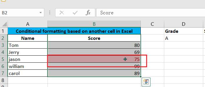
Step4: Excel will apply the selected format to the specific cell that meets the condition.

The method described above clearly does not meet our goal of highlighting the state of a specific column or other columns based on the value of a specific cell. That is, we need to format a specific cell or cell range in the Name column based on the value of cell E2.

When the built-in conditional rules of Excel or Google Sheets do not meet our goal, i.e., formatting other different cells based on a specific cell, then we need to use Excel or Google Sheets formulas to customize the formatting rules to meet our goal.

Below we will introduce how Microsoft Excel spreadsheet and Google Sheets respectively can customize conditional formatting rules via formulas to format cells in the Name column based on the value of cell E2.

Highlight Cells Based on Another Cell in Excel

If you want to highlight a cell range based on the value of another cell, then you can create custom conditional rules in Conditional Formatting. The specific steps are as follows.

Step1: Select the cell range where you want to apply the custom conditional rule, such as A2:B7

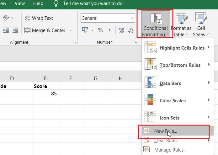
Step2: In the Ribbon area, select HOME->Conditional Formatting -> New Rule, the New Formatting Rule window will open.

Step3:  From below the list of rule types, we can see the type of rule we need, and that is we want to determine which cells to format by a formula. We need to select: Use a formula to determine which cells to format.

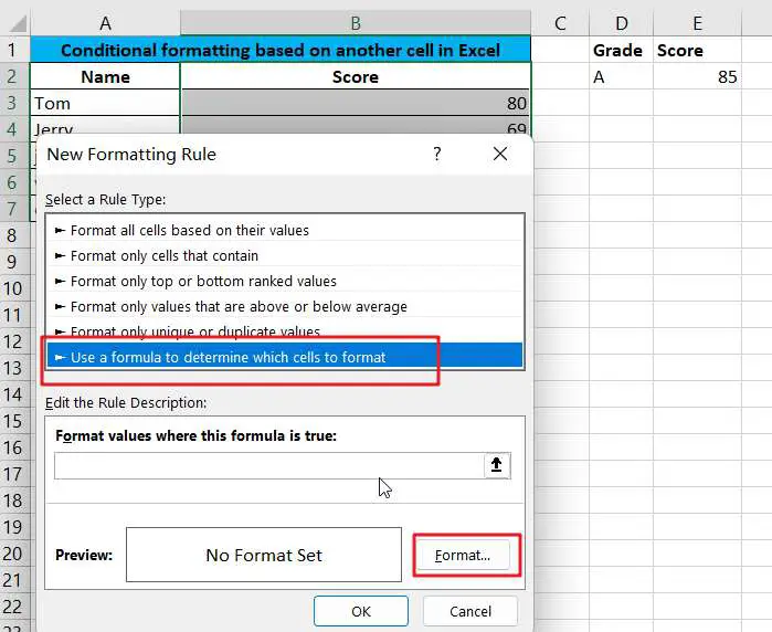
Note: As you can see from the image above, the New Formatting Rule dialog box has a number of rule types, such as, Format all cells based on their values, Format only cells that contain, Format only top or bottom ranked values, Format only values that are above or below average , Format only unique or duplicate values and Use a formula to determine which cells to format.

When the formatting formula is set to return a True value, the cell will apply the corresponding formatting, if the formula returns False, the formula will not be applied.

Step4: Enter the following formula in the Format values where this formula is true text box

=$B3>$E$2

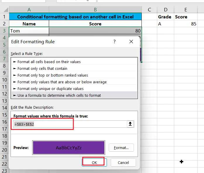
Note: As you can see from the formula above, cell E2 needs to use absolute references to limit cell changes, you need to enter the $ sign in front of the row and column values.

Step5: Click the “Format” button to select a format for the cells that meet the conditions.  

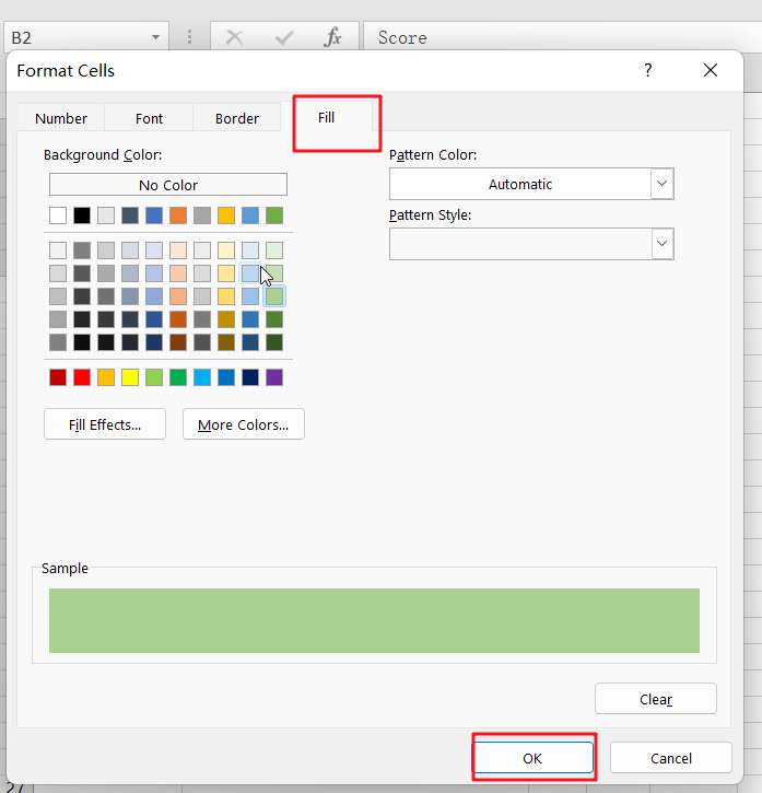
Step6: When you click OK, the selected format is applied to the cells that meet the conditions.

Highlight Cells Based on Another Cell in Google Sheets

The following is a conditional formatting function in the Google Sheet spreadsheet to highlight the cells in the name column that match the condition based on the cell’s value. The steps are as follows.

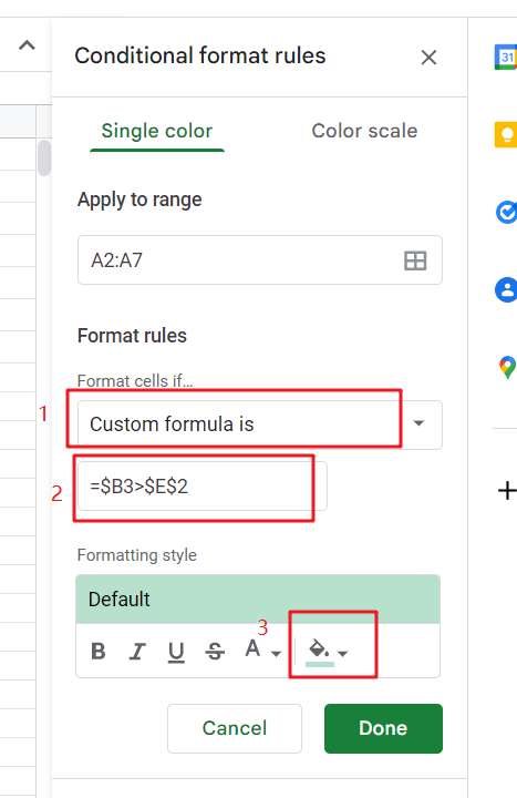
Step1: Select the cell range A3:A7 in the name column

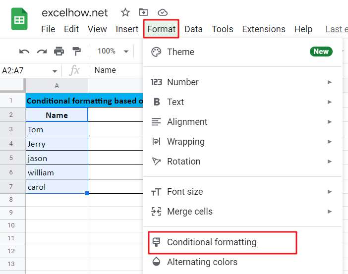
Step2: Click on the Format menu, and then click on the Conditional formatting menu

Step3: The Conditional formatting rules window will open.

Step4: Select Single color Tab

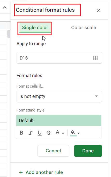
Step5: Select “Custom formula is” from the “Format Cells if” drop-down list

Step6: In the Formula text box, enter the following formula.

=$B3>$E$2

Step7: Select a style from the “Formatting style” drop-down list

Step8: Click on the “Done” button

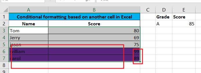
As you can see from the image above, you will see that the cell containing the name will be highlighted based on the score condition in the adjacent cell.

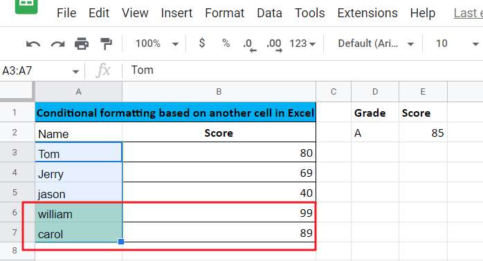
Note: When our custom conditional formula returns True, the cells that meet the condition will be formatted, when it returns False, google sheets will not do anything.

Multiple conditional rules

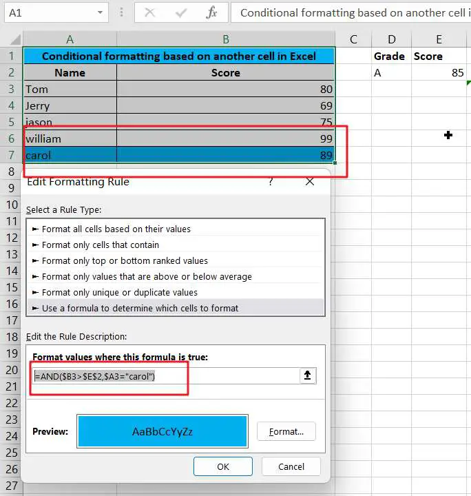
If you want cells that meet more than one condition to apply formatting, then you can use the logical functions AND and OR, for example, you want to highlight cells or ranges with a score greater than 90 and the name carol. Then you can use the following formula to customize the conditional rules.

=AND($B3>$E$2,$A3="carol")

The effect after applying the format is as follows.

Conditional Formatting Based On Another Cell FAQ

How do you conditionally format a cell based on another cell?

1. Select the cell you want to format…

2. On the Home tab, in the Styles group, click Conditional Formatting > New Rule…

3. In the New Formatting Rule window, select Use Formulas to Determine Which Cells Need to be Formatted.

4. Enter the formula in the appropriate box.

5. Click the “Format… ” button to select your custom format.

Can I use an IF formula in conditional formatting?

The answer is both yes and no. Any conditional formatting parameter must produce a “true” or “false” result, i.e., your conditional formatting rule is an If/Then statement that says “If this condition is “true”, format the cell in this way”.

Can you use conditional formatting based on relative cell references?

This cell reference type is rarely used in Excel conditional formatting rules.

Can you drag conditional formatting?

Yes, Select the cell and apply the conditional formatting, referencing other cells in the row. Drag the corner of the row down to the bottom of the cells you want to apply the formatting 

Video: Conditional Formatting Based On Another Cell in Excel/google sheets

Conclusion

Once you learn the conditional formatting function in Excel or Google Sheets, you will easily format other cells or ranges based on specific cell values, which is a is a very useful method.

SAMPLE FILES

Below are sample files in Microsoft Excel and google sheets that you can download for reference if you wish.