Suppose you come across a task where you need to calculate the average of the last 2 or 3 numeric values, then what would you do?
If you are new to Excel, then your first attempt might be doing this task manually, which is an acceptable way but only when the values of which you want to calculate the average is limited to 2 or 3 but when it comes to calculating the last 5 or N values in the columns then it becomes nearly impossible to do this cumbersome task on time!
Don’t worry about it because after reading this article, you will know the easiest way to calculate the average of the last 5 or N values from the columns within seconds.
So, let’s dive into the article.
Table of Contents
General Formula
To get the average of the last N values, use the formula below.
=AVERAGE(OFFSET(first cell,0,COUNT(range_values)-N,1,N))
Explanations For Syntax:
AVERAGE: In Excel, the AVERAGE Function may be used to calculate the arithmetic mean of a set of integers.OFFSET: This Function outputs a reference to a range made up of pieces such as a beginning point, a row, and column offset, and a final height and width in rows and columns. Learn more about the OFFSET Function.COUNT: The COUNT Function returns the result as a number and counts the number of cells that contain numbers.First Cell: It indicates the first cell in the provided input range.Range: This is the input value from your MS Excel spreadsheet.The comma sign (,): is a separator that separates a list of values.Parenthesis(): The main Function of this symbol is to group the elements.Minus Operator (-): This symbol subtracts 2 values.
Explanation
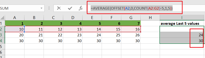
To average the latest 5 data values in a range of columns, use the AVERAGE Function conjunction with the COUNT and OFFSET functions. The formula in I2 in the example is as follows:
=AVERAGE(OFFSET(A2,0,COUNT(A2:G2)-5,1,5))
The OFFSET function may create dynamic ranges from a beginning cell and specify rows, columns, height, and width.
The rows and columns parameters act as “offsets” from the beginning reference. The height and width parameters, all optional, decide how many rows and columns are included in the final range. We want the OFFSET function to return a range that starts at the last item and grows “backward,” therefore we provide the following arguments:
A2 is the initial reference — it is the cell directly to the right of the formula and the first cell in the range of values we are dealing with.
Rows – We use 0 for the rows option because we want to stay in the same row.
Columns – We use the COUNT function to count all values in the range for the columns input, then deduct 5. This moves the start of the range of 5 columns to the left.
Height – we use 1 since we want a 1-row range as the end result.
Width – we pick 5 since we want a final range with 5 columns.
For the formula in I2, OFFSET yields a final range of C2:G2. This is sent to the AVERAGE Function, which returns the average of the five values in the range.
To understand better, consider the following example, which follows a step-by-step procedure:
- Consider the following example to calculate the average of the last 5 values.
- This illustration will provide input data from Column A to Column G.
- Next, enter the supplied formula in the formula bar section.
- Finally, we shall obtain the result in the selected cell I2.
Less Than 5 Values Average
If you are want to compute the average of the last 2, 3, or 4 data, you don’t need to do it manually. Utilizing the formula discussed above will result in a circular reference mistake when computing the average of the 2, 3, or 4 values in the columns; the range will extend back into the cell that contains the formula. To avoid this mistake and complete your task, modify the formula as follows:
=AVERAGE(OFFSET(first,0,COUNT(rng)-MIN(N,COUNT(rng)),1,MIN(N,COUNT(rng))))
So If you want to average last N values in columns that less than 5 values, you can use the following formula:
=AVERAGE(OFFSET(A2,0,COUNT(A2:C2)-MIN(5,COUNT(A2:C2)),1,MIN(5,COUNT(A2:C2))))
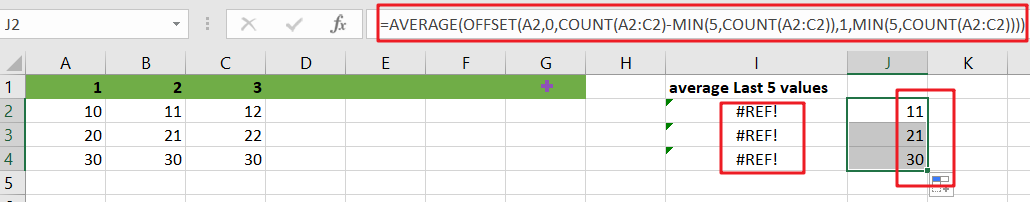
In this case, we utilize the MIN function to “catch” cases where there are fewer than 5 values and the real count when there are.
Related Functions
- Excel AVERAGE function
The Excel AVERAGE function returns the average of the numbers that you provided.The syntax of the AVERAGE function is as below:=AVERAGE (number1,[number2],…)…. - Excel COUNT function
The Excel COUNT function counts the number of cells that contain numbers, and counts numbers within the list of arguments. It returns a numeric value that indicate the number of cells that contain numbers in a range… - Excel MIN function
The Excel MIN function returns the smallest numeric value from the numbers that you provided. Or returns the smallest value in the array.The MIN function is a build-in function in Microsoft Excel and it is categorized as a Statistical Function.The syntax of the MIN function is as below:= MIN(num1,[num2,…numn])….