In Excel, INDEX function and MATCH function are often used together for returning value or cell reference or range reference from specified position. And MATCH function is one of Excel lookup & reference functions that can perform approximate match by setting match type.
Today, we will show you the basic usage of INDEX and MATCH through explaining a simple formula. This formula can also help you to get proper grade from Score-Grade table based on an input score. If you meet similar scenarios in your daily work, you can directly use this formula to deal with your problem.
Table of Contents
EXAMPLE
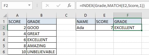
In this example, we want to get proper grade in F4 based on the entered score in F3. The relationship between score and grade you can refer to the left-side table. As the table only provides the starting score of each grade, so we can look up the entered score from this table “Score” column and return proper grade from “Grade” correspondingly by performing an approximate match.
Before creating a formula to solve this problem, to illustrate the formula, we defined three named ranges “Score” (A2:A6) and “Grade” (B2:B6). In this article, to approach our goal, we will apply INDECT & MATCH functions to create formula.
ANALYSIS
To return proper grade based on score entry:
1. There is only one condition to determine the returned grade: score.
2. In this example, our input score is “7” which is not listed directly in range “Score”, and “Score” only provides the starting scores for each grade, so we can only find the starting score of input score “7” through performing an approximate match.
3. Through locating the starting score of “7” from named range “Score”, we can return grade for this starting score correspondingly from adjacent column “Grade”.
In Excel, INDEX and MATCH functions are good partners for searching. MATCH function can return the position based on searching for specific content, and INDEXT can query the corresponding data according to the position. In this example, MATCH function returns proper position of starting score based on the given score in E2, then INDEX function returns grade based on the position.
Above all, we create below formula to solve this problem:
=INDEX(Grade,MATCH(E2,Score,1))
FORMULA
Input formula =INDEX(Grade,MATCH(E2,Score,1)) into F2, press ENTER, verify that “EXCELLENT” is returned properly.
In Excel, refer to approximate match rules, score in “Score” column is the starting value for corresponding grade. As “EXCELLENT” is the grade for score which is greater than or equal to 6, “AMAZING” is for score which is greater than or equal to 8, so “EXCELLENT” is correct for score 7. More details please see below Explanation part.
FUNCTION INTRODUCTION
a. INDEX function returns a value or a reference based on given cell or range reference.
For array form:
Syntax:
=INDEX(array, row_num, [column_num])
For reference form:
Syntax:
=INDEX(reference, row_num, [column_num], [area_num])
There are two forms of INDEX functions. You can apply array form if the first argument to INDEX is an array constant. And usually INDEX returns reference of the intersection of a particular row and column when applying INDEX with reference form.
b. MATCH function returns the relative position of a cell from a range which cell contains specific item.
Syntax:
=MATCH(lookup_value, lookup_array, [match_type])
EXPLANATION
=INDEX(Grade,MATCH(E2,Score,1))

//
for MATCH, lookup_value is E2 (7),lookup_array is named range “Score”, match_type is “1”
//
for INDEX, array is named range “Grade”, row number is MATCH function return value
a. In MATCH(E2,Score,1), expand values in arguments:
=MATCH(7,{2;4;6;8;10},1)
//
expand values in E2 and named range “Score”
b. For match type, there are three values “0”, “1”, and “-1”. The default value is “1”. If we set match type to “1”, MATCH function finds out all values that are less than or equal to lookup_value from lookup_array, and returns the largest one among them, that means MATCH function performs an approximate match when setting match type to “1”.
In this example, as lookup_value is “7”, so from lookup_array only numbers “2”, “4” and “6” can meet the rule, “6” is the largest one. For starting score “6”, for the entire worksheet, its row number is 4; but MATCH function returns its relative position in range “Score” (A2:A6), so its row number is 3.
c. “3” is delivered to INDEX as row number.
=INDEX(Grade,3)
//
row number is 3 for starting value “6”
Expand values in “Grade”.
=INDEX({"GOOD";"GREAT";"EXCELLENT";"AMAZING";"UNBELIEVABLE"},3) //
returns “EXCELLENT”
Related Functions
- Excel INDEX function
The Excel INDEX function returns a value from a table based on the index (row number and column number)The INDEX function is a build-in function in Microsoft Excel and it is categorized as a Lookup and Reference Function.The syntax of the INDEX function is as below:= INDEX (array, row_num,[column_num])… - Excel MATCH function
The Excel MATCH function search a value in an array and returns the position of that item.The MATCH function is a build-in function in Microsoft Excel and it is categorized as a Lookup and Reference Function.The syntax of the MATCH function is as below:= MATCH (lookup_value, lookup_array, [match_type])….