Microsoft Excel provides many functions that can execute logical test, search data, return current date and something else. They are very useful in daily work. And Excel VLOOKUP function is one of Excel most frequently used functions. It belongs to lookup & reference functions and it can perform approximate match or exact match by setting lookup matching modes accordingly.
Today, we will show you the way to calculate “Rates” based on input weight by VLOOKUP function. In this instance, VLOOKUP will perform an approximate match when scanning the lookup value from the given table. If you meet similar scenarios in your daily work, you can directly use the formula we created in this case to deal with your problem.
EXAMPLE
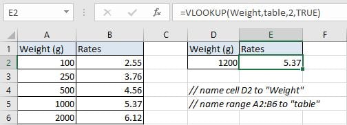
In this example, we want to know the corresponding rates for the input weight “1200” in E2. The corresponding relationship between weights and rates are saved in range (A2:B6), weights are listed in the first column and rates are listed in the second column of this table. As the table only provides the starting value of each weight band, if the input weight cannot be found in the first column, we should perform an approximate match and find the approximation of the input weight. Above all, we need to create formula that can look up the input weight in the first column of the given table, and also can perform an approximate match if the input weight cannot be found, at last it can return proper rates from the second column based on searching result.
In precondition, name cell D2 to “weight”, name range A2:B6 to “table”.
In this article, to approach our goal, we will apply VLOOKUP function to create formula.
ANALYSIS
To return proper rates based on the input weight:
- Which value returns depends on the input weight (weigh band).
- In this example, our input weight is “1200”, it is not listed in “Weight” column, but refer to the given table, we can know that it belongs to the weight band 1000-1999g. So, we need to scan each weight from “Weight” column and compare with the input weight, then find out the position of the starting weight of weight band “1000-1999g” by performing an approximate match.
- After confirming the starting weight, the formula should return corresponding rates value from adjacent “Rates” column properly.
In Excel, except the good partners INDEX and MATCH, we can also select some other functions to look up values. VLOOKUP is one of the most frequently used functions in Excel that can perform searching data properly, it also can perform approximate match or exact match by setting match mode.
Above all, we create below formula to solve this problem:
=VLOOKUP(Weight,table,2,TRUE)
FORMULA
Input formula =VLOOKUP(Weight,table,2,TRUE) into E2, press ENTER, verify that “5.37” is returned properly.
Values in “Weight” column are the starting weight for each weight band. Refer to normal approximate match rules, rates “5.37” is the corresponding to weight band “1000-1999g”, rates “6.12” is corresponding to weight band “2000+”, so “5.37” is returned for input weight 1200g. More details please see below Explanation part.
FUNCTION INTRODUCTION
a. VLOOKUP function looks up the input value from the first column of the given table, and returns the value we want from a particular position (row number depends on the row of lookup value, column number depends on the input argument col_index_num).
Syntax:
=VLOOKUP(lookup_value, table_array, col_index_num,[range_lookup])
For argument “range_lookup”, there are two matching modes “True” and “False”.
- The default mode is “True”, so if this optional argument is omitted, this value is set to “True” automatically.
- If we set “range_lookup” to “True”, VLOOKUP function performs an approximate match.
- If we set “range_lookup” to “False”, VLOOKUP function looks up data restrictively by performing an exact match. If look up value is not found in table, formula returns error “#N/A”.
EXPLANATION
=VLOOKUP(Weight,table,2,TRUE)
lookup_value is the weight input into cell reference “Weight”
table_array is named range “table”(A2:B6)
col_index_num is 2. Because rates are saved in the second column of this table.
range_lookup is set to TRUE. VLOOKUP function performs an approximate match.
a. In this formula, the look up value is “1200”, VLOOKUP scans this value from the first column of the given table, in this case it is the range “A2:A6”. It continues scanning until it meets the value that is greater than the lookup value. In this case, VLOOKUP function will stop scanning when meeting “2000” and returns to previous row. In this example, it returns to A5.
b. The given table_array is range “A2:B6”, this table contains the lookup value in its first column and also contains the rates we want to return by the formula, so we input “A2:B6” as table_array, just input a single column doesn’t work.
c. As the rates are listed in the second column of A2:B6, so we enter 2 as col_index_num. VLOOKUP function retrieves data at the position that next to A5 in the second column, in this example value lists in B5 is 5.37.
EXPAND
a. We can also create below formula contains INDEX and MATCH to help us solve the problem:
=INDEX(B2:B6,MATCH(Weight,A2:A6,1))
b. When performing an approximate match of VLOOKUP function, the lookup values must be sorted in ascending order in precondition. If values in the first column are in disorder, VLOOKUP function will stop scanning if it meets the first value that is greater than the lookup value, thus the returned value is improper.
Related Functions
- Excel INDEX function
The Excel INDEX function returns a value from a table based on the index (row number and column number)The INDEX function is a build-in function in Microsoft Excel and it is categorized as a Lookup and Reference Function.The syntax of the INDEX function is as below:= INDEX (array, row_num,[column_num])… - Excel MATCH function
The Excel MATCH function search a value in an array and returns the position of that item.The MATCH function is a build-in function in Microsoft Excel and it is categorized as a Lookup and Reference Function.The syntax of the MATCH function is as below:= MATCH (lookup_value, lookup_array, [match_type])…. - Excel VLOOKUP function
The Excel VLOOKUP function lookup a value in the first column of the table and return the value in the same row based on index_num position.The syntax of the VLOOKUP function is as below:= VLOOKUP (lookup_value, table_array, column_index_num,[range_lookup])….