In Excel, except combination INDEX+MATCH, we can also apply other functions to search data, for example VLOOKUP function. Like MATCH function, VLOOKUP function is one of Excel lookup & reference functions that can perform approximate match or exact match by setting lookup matching modes.
Today, we will show you the way to calculate discount by VLOOKUP function. In this instance, VLOOKUP will perform an approximate match when scanning values from the given table. If you meet similar scenarios in your daily work, you can directly use the formula with the help of VLOOKUP function we created in this case to deal with your problem.
Table of Contents
EXAMPLE
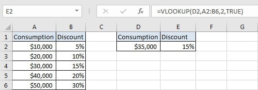
In this example, we want to define a formula in E2 that can return a discount based on the input consumption in D2 correspondingly. The corresponding relationship between consumption and discount are listed in the left table. As the table only provides the consumption starting value for each discount, so we can look up the input consumption from this table, and return proper discount correspondingly by performing an approximate match.
In this example, we want to define a formula to return the discount. In fact, there are many Excel lookup & reference functions of functions combination that can solve this problem. This formula must can look up the input value (in D2) from the given table (A2:B6), performances an approximate match and retrieves data from a particular position properly.
In this article, to approach our goal, we will apply VLOOKUP function to perform an approximate match to return a proper discount.
ANALYSIS
To return discount based on the input consumption:
1. There is only one condition to determine the returned discount: the input consumption.
2. In this example, our input consumption “35000” is not listed in “Consumption” column, so we need to make sure that the input value belongs to which consumption range, and confirm the starting value of this range. So, we need to select a function that can perform an approximate match to create the formula.
3. Based on the starting value, we can find the discount in the adjacent column. So, we need to select a function that can retrieve data at a particular position.
There are several lookup & reference related functions that can meet above conditions, in this article we select VLOOKUP function to figure out this issue. Create a formula with VLOOKUP function:
=VLOOKUP(D2,A2:B6,2,TRUE)
FORMULA
Input formula =VLOOKUP(D2,A2:B6,2,TRUE) into E2, press ENTER, verify that “15%” is returned properly.
FUNCTION INTRODUCTION
a. VLOOKUP function looks up the input value from the first column of the given table, and returns the value we want from a particular position (row number depends on the row of lookup value, column number depends on the input argument col_index_num).
Syntax:
=VLOOKUP(lookup_value, table_array, col_index_num,[range_lookup])
For argument “range_lookup”, there are two matching modes “True” and “False”.
- The default mode is “True”, so if this optional argument is omitted, this value is set to “True” automatically.
- If we set “range_lookup” to “True”, VLOOKUP function performs an approximate match.
- If we set “range_lookup” to “False”, VLOOKUP function looks up data restrictively by performing an exact match. If look up value is not found in table, formula returns error “#N/A”.
EXPLANATION
=VLOOKUP(D2,A2:B6,2,TRUE)
lookup_value is input into D2 (“35000”)
table_array is “A2:B6”,
col_index_num is 2. Because discounts are saved in the second column of this table.
range_lookup is set to TRUE. So VLOOKUP function performs an approximate match.
a. In this formula, the look up value is “$35,000”, VLOOKUP scans this value from the first column of the given table, in this case it is the range “A2:A6”. It continues scanning until it meets the value that is greater than the lookup value. In this case, VLOOKUP function will stop scanning when meeting $40,000 and returns to previous row of “$30,000”.
b. The given table_array is range “A2:B6”, this table should contain the lookup value in its first column and also contains the discount we want to return by the formula, so we input “A2:B6” as table_array, just input a single column doesn’t work.
c. As the discounts are listed in the second column of A2:B6, so the col_index_num is 2. So, VLOOKUP function retrieves data at the intersection of the second column and the row of “$30,000”.
EXPAND
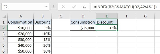
a. We can also use the combination INDEX + MATCH to return discount. In Excel, INDEX function and MATCH function are often used together for returning value or cell reference/range reference from a particular position.
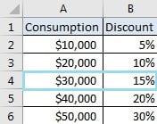
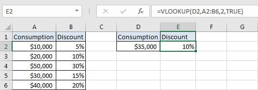
b. When performing an approximate match of VLOOKUP function, the lookup values must be sorted in ascending order in precondition. If values in the first column are in disorder, VLOOKUP function will stop scanning if it meets the first value that is greater than the lookup value, thus the returned value is improper. See example below.
Related Functions
- Excel INDEX function
The Excel INDEX function returns a value from a table based on the index (row number and column number)The INDEX function is a build-in function in Microsoft Excel and it is categorized as a Lookup and Reference Function.The syntax of the INDEX function is as below:= INDEX (array, row_num,[column_num])… - Excel MATCH function
The Excel MATCH function search a value in an array and returns the position of that item.The MATCH function is a build-in function in Microsoft Excel and it is categorized as a Lookup and Reference Function.The syntax of the MATCH function is as below:= MATCH (lookup_value, lookup_array, [match_type])…. - Excel VLOOKUP function
The Excel VLOOKUP function lookup a value in the first column of the table and return the value in the same row based on index_num position.The syntax of the VLOOKUP function is as below:= VLOOKUP (lookup_value, table_array, column_index_num,[range_lookup])….