AVERAGE function is one of the most popular functions in Excel. Apply AVERAGE together with some other functions, we can calculate average simply for some complex situations.
In this article, we will introduce you to calculate average of the last N numbers from a range contains both numeric values and non-numeric values.
Table of Contents
EXAMPLE
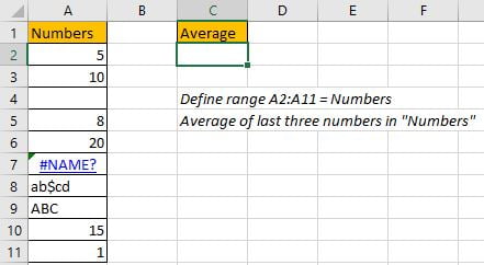
In this case, we want to calculate the average of the last 3 numeric values in “Numbers” column. As non-numeric value “ABC” exists in last three cells, so we cannot directly apply AVERAGE(A9:A11) directly. To calculate average ignoring invalid values, we need the help of other functions.
In this article, to approach our goal, except the main AVERAGE function, we also apply ROW, ISNUMBER, IF, LARGE, LOOKUP functions.
SOLUTION
To create a formula to get average in this case, we need to know:
1) Distinguish numbers and non-numeric values from range “Numbers”. Ignore non-numeric values in calculation.
2) Find out the last three cells with numbers in “Numbers”.
3) Find out last three values through searching for the last three positions.
FORMULA with AVERAGE & OTHER FUNCTIONS
In C2, we input the formula
=AVERAGE(LOOKUP(LARGE(IF(ISNUMBER(Numbers),ROW(Numbers)),{1,2,3}), ROW(Numbers), Numbers)).
After typing, press Enter, average of the last three numbers is 12.
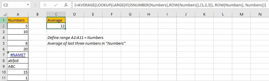
In “Numbers” list, the last three values are 20, 15 and 1, the average is (20+15+1)/3=12, so the formula returned value is correct. The last three values are found out properly.
FUNCTION INTRODUCTION
The main function in this formula is “AVERAGE”, it can return the average of last three values; Others are supported to find out numbers (ignoring non-numeric values), mark row numbers for the last three numbers, and the through searching row numbers to return corresponding numbers.
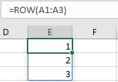
1. ROW function returns row number for a given range reference.
Syntax:
=ROW(reference)
Example. ROW(A1:A3) returns row numbers of range A1:A3, so we get {1;2;3}.
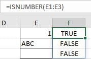
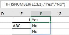
2. ISNUMBER function returns True (for numeric values) or False (for strings, errors) based on value is a numeric value or not. For blank cells, it returns False.
Syntax:
=ISNUMBER(value)
Example. You can input a value, a cell reference, or a range reference for “value”.
3. IF function returns “true value” or “false value” based on the result of provided logical comparison. It is one of the most popular function in Excel.
Syntax:
=IF(logical_test,[value_if_true],[value_if_false])
Example, =IF(ISNUMBER(E1:E3),”Yes”,”No”).
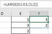
4. LARGE function returns the Kth largest number from a given set of numbers or a range reference.
Syntax:
=LARGE(array,k)
Example, =LARGE(E1:E3,{1;2}), an array {3;2} is returned. If you set k=2, only 2 is returned.
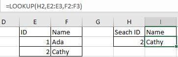
5. LOOKUP function can through searching for a row or column to return the corresponding value in the same position but in the second row or column. It has two different syntaxes, in this case, it is for vector:
Syntax:
=LOOKUP(lookup_value, lookup_vector, [result_vector])
Example, =LOOKUP(H2,E2:E3,F2:F3), apply lookup to find out name for id1.
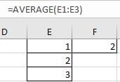
6. AVERAGE function returns the average of numbers from a given range reference.
Syntax:
=AVERAGE(number1, [number2], …)
Example. For arguments “number1, number2,…”, they can be a set of numbers, or an array of numbers like {1;2;3}.
FORMULA EXPLANATION
=AVERAGE(LOOKUP(LARGE(IF(ISNUMBER(Numbers),ROW(Numbers)),{1,2,3}), ROW(Numbers), Numbers))
This formula contains 6 functions, we explain functions from inside to outside.
1. For ISNUMBER(Numbers), “Numbers” is A2:A11, so ISNUMBER function check values in each cell in this range and returns “True” for numeric values and “False” for non-numeric values or blank. ISNUMBER(Numbers) returns below array:
{TRUE;TRUE;FALSE;TRUE;TRUE;FALSE;FALSE;FALSE;TRUE;TRUE}
2. ROW(Numbers)
returns row numbers for range A2:A11.
{2;3;4;5;6;7;8;9;10;11}
3. With the help of ISNUMBER and ROW functions, IF function returns row numbers for cells with numeric values.
IF({TRUE;TRUE;FALSE;TRUE;TRUE;FALSE;FALSE;FALSE;TRUE;TRUE},{2;3;4;5;6;7;8;9;10;11})
Based on logical test result, IF returns row number for “true value” and keeps “False” for “false value” as [value_if_false] is omitted. Then we get below array from IF function:
{2;3;FALSE;5;6;FALSE;FALSE;FALSE;10;11}
4. Now above array returned from IF function participates into LARGE function calculation.
LARGE({2;3;FALSE;5;6;FALSE;FALSE;FALSE;10;11},{1,2,3})
K is an array {1,2,3}, so LARGE function returns the largest three values from array {2;3;FALSE;5;6;FALSE;FALSE;FALSE;10;11}. In this step, LARGE function returns the last three row numbers for cells with numbers.
{11,10,6}
5. In step#4, we get the last three row numbers properly. Then we can apply LOOKUP function to lookup corresponding values in row 11, row 10 and row 6 from range “Numbers”.
Row(Numbers) is applied twice in this formula, the first one is “value_if_true” for IF function, the second one is used as “lookup_vector” for LARGE function.
LOOKUP({11,10,6}, ROW(Numbers), Numbers)=LOOKUP({11,10,6}, {2;3;4;5;6;7;8;9;10;11}, {5;10;0;8;20;#NAME?;"ab$cd";"ABC";15;1})
In this step, LOOKUP function returns proper values from A2:A11 after searching for row numbers 11, 10 and 6. So we get below array at last:
{1,15,20}
6. After above all steps, we get =AVERAGE({1,15,20}). So, the returned value is (1+15+20)/3=12.
Related Functions
- Excel ROW function
The Excel ROW function returns the row number of a cell reference.The ROW function is a build-in function in Microsoft Excel and it is categorized as a Lookup and Reference Function.The syntax of the ROW function is as below:= ROW ([reference])…. - Excel IF function
The Excel IF function perform a logical test to return one value if the condition is TRUE and return another value if the condition is FALSE. The IF function is a build-in function in Microsoft Excel and it is categorized as a Logical Function.The syntax of the IF function is as below:= IF (condition, [true_value], - Excel ISNUMBER function
The Excel ISNUMBER function returns TRUE if the value in a cell is a numeric value, otherwise it will return FALSE.The syntax of the ISNUMBER function is as below:= ISNUMBER (value)… - Excel LOOKUP function
The Excel LOOKUP function will search a value in a vector or array.The syntax of the LOOKUP function is as below:= LOOKUP (lookup_value, lookup_vector, [result_vector])…
- Excel AVERAGE function
The Excel AVERAGE function returns the average of the numbers that you provided.The syntax of the AVERAGE function is as below:=AVERAGE (number1,[number2],…)…. - Excel LARGE function
The Excel LARGE function returns the largest numeric value from the numbers that you provided. Or returns the largest value in the array. The syntax of the LARGE function is as below:= LARGE (array,nth)…