In Excel, INDEX function and MATCH function are often used together for returning data from specific position. And MATCH function is one of Excel lookup & reference functions that can return approximate value by setting match type. Above all, through generating a formula with INDEX and MATCH function, we can get an approximate value properly based on given data and cell or range reference.

In this article, through explaining the example below, we will introduce you the formula with INDEX and MATCH used that can help you returning approximate value. If you meet similar scenarios in your daily work, you can directly use it.

EXAMPLE

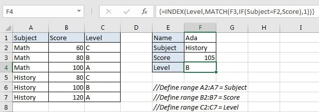
In this example, we want to get return level in F4 based on two entries “subject” in F2 and “score” in F3. As there is no definition to explain the scope of level A, B and C exactly, so we can lookup entered score from named range “Score” and return an approximate level from “Level” correspondingly.

For different subjects, the correspondences between score and level are different. For math, for score of 60, we can get a C-level, but for history, you cannot get a C-level until you get a score of 80. So, to return a proper approximate level from “Level”, except the entered score, we also need to lookup subject from range “Subject”, then return level based on this subject’s score-level correspondence.

Before creating a formula to solve this problem, in order to illustrate the formula, we defined three named ranges “Subject” (A2:A7), “Score” (B2:B7), and “Level” (C2:C7). In this article, to approach our goal, we will apply INDECT & MATCH functions to create formula, with the help from IF function inside as argument.

ANALYSIS

To return level based on input subject and score:

1. There are two conditions to determine the returned level: subject and score.

2. As “History” can be found from named range “Subject”, so we can through searching for “History” (in F2) from named range “Subject” to get score and level corresponding relationship.

3. Through locating a score from named range “Score”, we can get a level for this score correspondingly.

4. In this example, there is no level for score “105” exactly. So, we can only return an approximate level based on the two entries refer to the corresponding relationship between score and level in above table.

In Excel, INDEX and MATCH functions are good partners for searching. MATCH function can return the position based on searching for specific content, and INDEXT can query the corresponding data according to the position. In this example, MATCH function returns proper position of score for subject “History”, and INDEX function can return proper level based on the position.

With the help from IF function, we create below formula to solve this problem:

=INDEX(Level,MATCH(F3,IF(Subject=F2,Score),1))

 FORMULA

Input formula =INDEX(Level,MATCH(F3,IF(Subject=F2,Score),1)) into F4, as this is an array formula, so press Ctrl+Shift+Enter, verify that level B is returned properly.

In Excel, refer to approximate match rules, score in “Score” column is the starter value for corresponding level. As level B is for score which is greater than or equal to 100, level A is for score which is greater than or equal to 120, so we think level B is correct for score 105. More details please see explanation part.

FUNCTION INTRODUCTION

a. INDEX function returns a value or a reference based on given cell or range reference.

 For array form:

Syntax:

=INDEX(array, row_num, [column_num])

 For reference form:

Syntax:

=INDEX(reference, row_num, [column_num], [area_num])

 There are two forms of INDEX functions. We apply array form as the first argument to INDEX is an array constant. Usually INDEX returns reference of the intersection of a particular row and column when applying INDEX with reference form.

 b. MATCH function returns the relative position of a cell from a range which cell contains specific item.

Syntax:

MATCH(lookup_value, lookup_array, [match_type])

 

c. IF function returns “true value” or “false value” based on the result of provided logical test. It is one of the most popular function in Excel.

Syntax:

=IF(logical_test,[value_if_true],[value_if_false])

EXPLANATION

=INDEX(Level,MATCH(F3,IF(Subject=F2,Score),1))

// for IF, logical test “Subject=F2”, value_if_true is named range “score”, value_if_false is omitted  

// for MATCH, lookup_value is F3 (105),lookup_array is IF function return value, match_type is “1”

// for INDEX, array is named range “Level”, row number is MATCH function return value

 a. The formula’s core functions are INDEX and MATCH, but IF function can help us list all scores for subject “History”. In logical test argument, we input “Subject=F2” as we are looking for history from “Subject”. Expand values in “Subject” and “Score”, we get below expression:

IF({"Math";"Math";"Math";"History";"History";"History"}="History",{60;80;100;80;100;120})

If values in array {“Math”;”Math”;”Math”;”History”;”History”;”History”} match “History”, then corresponding values from array {60;80;100;80;100;120} are returned. So, we get below array after running IF function.

{FALSE;FALSE;FALSE;80;100;120}

 b. IF function returned array is delivered to MATCH function as lookup_array. Now, in MATCH(F3,IF(Subject=F2,Score),1), lookup_value is F3 “105”, lookup_array is {FALSE;FALSE;FALSE;80;100;120}, match_type is “1”.

For match type, there are three values “0”, “1”, and “-1”. The default value is “1”. If we set match type as “1”, Match function finds out all values that are less than or equal to lookup_value from lookup_array, and returns the largest one among them.

In this example, as lookup_value is 105, so from lookup_array only 80 and 100 meet the rule, 100 is larger than 80, so the relative position of cell B6 which contains “100” for subject history is returned from MATCH function. In named range “Score” (B2:B7), “100” is saved in B6, so the relative row number is 5 (the first value is started in row2).

 c. “5” is delivered to INDEX as row number.

INDEX(Level,5) // row number is 5 for “100”

 Expand values in “Level”, INDEX returns “B” finally.

=INDEX({“C”;”B”;”A”;”C”;”B”;”A”},5)

//

returns “B”

Related Functions

---

• Excel INDEX function
  The Excel INDEX function returns a value from a table based on the index (row number and column number)The INDEX function is a build-in function in Microsoft Excel and it is categorized as a Lookup and Reference Function.The syntax of the INDEX function is as below:= INDEX (array, row_num,[column_num])…
• Excel MATCH  function
  The Excel MATCH function search a value in an array and returns the position of that item.The MATCH function is a build-in function in Microsoft Excel and it is categorized as a Lookup and Reference Function.The syntax of the MATCH function is as below:= MATCH  (lookup_value, lookup_array, [match_type])….
• Excel IF function
  The Excel IF function perform a logical test to return one value if the condition is TRUE and return another value if the condition is FALSE. The IF function is a build-in function