Still cannot understand the functions and formulas in Excel or google sheets and trouble? The most basic excel or google sheets function parameters introduction, newcomers must see!
Table of Contents
ABSTRACT
Our website introduces many basic uses of functions in Excel or google sheets as well as common examples from everyday life and work. We have also uploaded many articles on how to use functions to create formulas to solve common problems.
We found that, in fact, many people do not know much about Excel or google sheets functions, or a half-understanding, by reading our articles may solve the current problem, but they do not know how to use Excel or google sheets functions to create formulas when solving the problem, with what function? Which similar function to use? How to nest the formula? What is the input value? Why does it return an error?
We will have the above problems because we usually only think about how to quickly apply these functions as well as formulas to solve problems in a timely manner, and copy the formula directly to use it without thinking about how the formula works.
We will face a lot of problems, so before we learn Excel or google sheets functions and formulas, we must learn some basic concepts about functions and formulas, or a few basic elements that make up a function/formula. Then after understanding these basic concepts, you will really see how a formula is made up and what role each part plays in the formula.
– Arguments
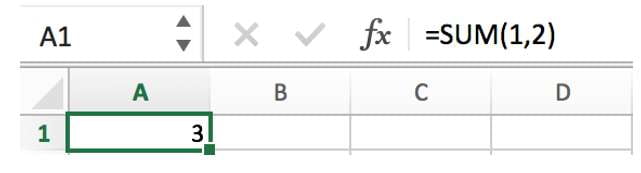
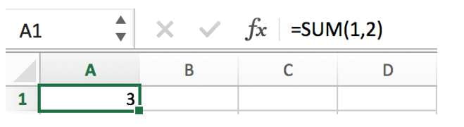
Referring to the syntax structure of the function, each item in the function brackets is called an argument to the function. These arguments can be constants, cell reference, range reference, arrays, nested functions, etc. Next, we will introduce them according to different categories of arguments.
In the example below, number 1 and 2 are arguments to SUM function.
– Constants
Constant is an immutable value or data item. A constant can be a specified value, array, or character/string. In a normal Excel or google sheets formula, in addition to the value itself, you can also enter a cell reference or range reference that contains the value(s).
Note: Neither the formula nor the result calculated by the formula is a constant, because whenever the argument of the formula changes, it will affect the formula calculation and change the result.
In the example below, arguments 1 and 2 are entered manually, they are constants.
– Cell Reference & Range Reference
Cell reference and cell range reference are the most common arguments in Excel or google sheets functions. The purpose of the reference is to define the cell or range in the worksheet and specify the location of the data used by the formula or function, so that the function can easily use the data in various parts of the worksheet.
The values in cell references and range references can be static values, but they can also be dynamic values. The actual return value according to the change in the value of cell reference or range reference.
Cell Reference
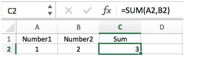
In the example below, A2 and B2 are cell references. Number “1” is saved in cell reference A2, “2” is saved in cell B2. When selecting A2 in a function, that means number “1” in A2 is referenced.
A cell reference is delivered to function as its argument.
Range Reference
The entire selected multiple cells can be seen a range reference. In Excel or google sheets, for the common used lookup function VLOOKUP, its lookup range argument is usually entered with a range reference.
In the example below, A2:B2 is a range reference, it is one argument to SUM function not two arguments. This range reference contains an array actually. We will introduce array in the following paragraph.
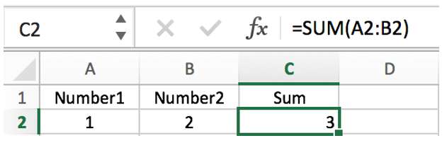
When entering or typing function’s arguments, we can click on a single cell, or drag and drop to select multiple cells, in this way we can directly enter a cell reference or range reference.
We can also pre-define a name for a range reference in advance, in this way, we can enter this name directly as function’s argument when applying a function.
STEP 1: Name a range reference:
Formulas->Define Name, enter “Numbers” for selected range:
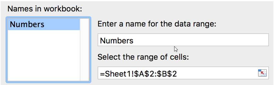
OR
Select A1:B2->Enter “Numbers” in Name Box:
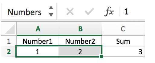
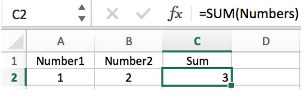
STEP 2: Entering “Numbers” as argument.
As functions or formulas are often copied directly to other cells through drag-and-drop operations, usually, the reference will change automatically according to the cell location where the formula is located.
If you do not want to change the reference, we must add a dollar sign in front of the row or column index. For these two cases, we divided the reference into relative reference and absolute reference.
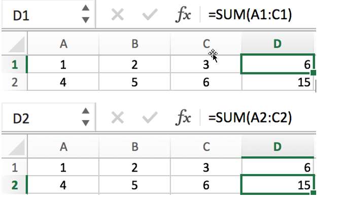
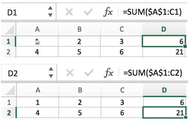
Relative Reference:
When dragging down the formula, A1:C1 is automatically updated to A2:C2.
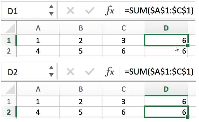
Absolute Reference:
When dragging down the formula, $A$1:$C$1 is not changed. Because we add $ before row and column indexes, so range reference is locked.
Mixed Reference:
When dragging down the formula, for range reference $A$1:C1, $A$1 is locked, but C1 is updated from C1 to C2 as formula is copied down to D2.
– Array
Array, equivalent to our mathematical matrix, a matrix contains multiple elements, elements and different combinations of elements constitute a matrix of different dimensions.
In EXCLE workbook, the selected range can be expressed as an array, expressed as an N row * M column area, N and M are not 0.
The array formula is relative to the ordinary function formula; it has two characteristics.
1) Elements of the array are referenced by brackets {} and separated by commas or semicolons.
2) After entering an array formula, you must press Ctrl+Shift+Enter to load the result.
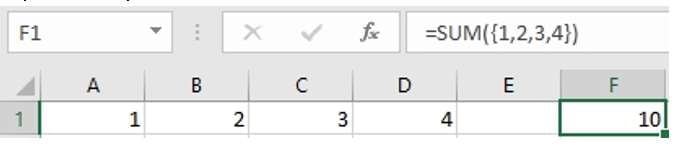
Example 1:
F1=SUM(A1:D1); A1:D1={1,2,3,4}; If all elements in on array are in one row, values are separated by comma.
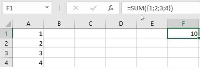
Example 2:
F1=SUM(A1:A4); A1:A4={1;2;3;4}; If all elements in on array are in one column, values are separated by semicolon.
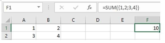
Example 3:
F1=SUM(A1:B2); A1:B2={1,2;3,4}; The array is a multidimensional array.
– Logical Values
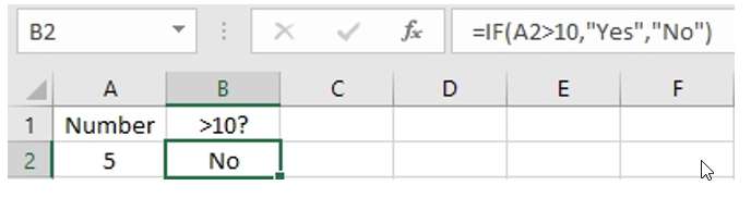
There are TRUE and FALSE two logical values. In Excel or google sheets, IF function is a logical test function that returns the corresponding branch value based on the two logical values TRUE and FALSE.
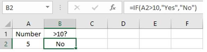
Example:
If logical test value is TRUE, IF function returns “Yes” else returns “No”.
– Logical Operators
AND
Syntax: AND(logical1, logical2, …).
Description: Returns TRUE if all arguments are true; and If AND function detects an argument with a value of false, it returns false
Example:
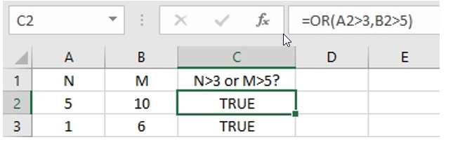
If both conditions “N>3” and “M>5” are true, result is TRUE.
NOT
Syntax: NOT(logical)
Description: Find the opposite of a logical value or a logical expression. If you want to get the opposite of a logical value, you should use the NOT function.
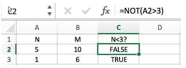
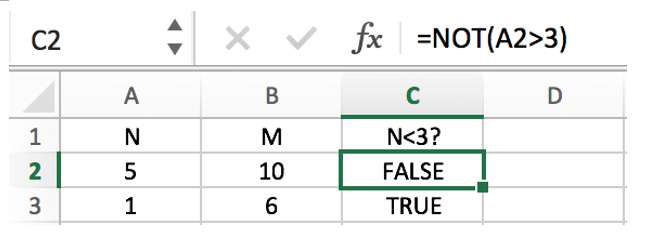
Example:
Normally we can use IF function to create a logical test like =IF(A2>3,”TRUE”,”FALSE”) to return TRUE or FALSE result; Actually you can make it easier, you can also use “=NOT(A2>3)” to return the result of logical test “N<3”.
OR
Syntax: OR(logical1, logical2, …)
Description: Returns TRUE when any of the logical values is true.
Example:
If one of the conditions “N>3” and “M>5” is true, result is TRUE.
IF
The IF function is used to make logical judgments
Syntax: IF(logical_test, value_if_true, value_if_false)
Description: IF function performs a logical test which can return different results depending on the TRUE or FALSE of the logical expression.
Example:
Set “Yes” to logical test value of TRUE; Set “No” to logical test value of FALSE.
– Error Values
Sometimes we don’t get the value we want after pressing the Enter key, and formula returns error value instead. These values usually consist of “#error!”.
When we find that an error is returned, we need to understand the meaning of these errors, they can help us to know what the cause of the error is and how to solve the error.
Below is a list of common error values and solutions in Excel or google sheets function applications.
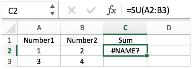
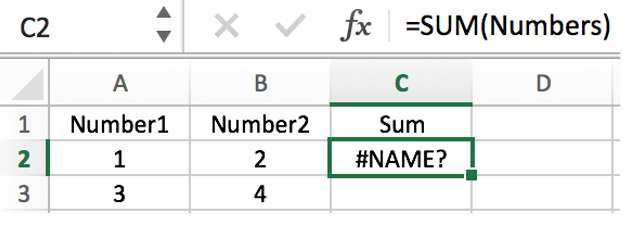
Error: #NAME?
Explanation: The function was entered incorrectly with unrecognized text. For example, the function name is spelled incorrectly, the quoted text is not quoted, and so on.
Solution: Check for spelling errors, quotation marks and brackets
Example1: Function name “SUM” is spelled incorrectly
Example2: Reference “Numbers” is missing
Error: #N/A
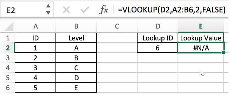
Explanation: The lookup range cannot be found when using some lookup functions in Excel workbook (for example, the VLOOKUP function cannot find the input lookup range, or the lookup value cannot be found in the first column of the lookup range).
Solution: Check if the lookup range has been entered incorrectly; make sure the lookup value is in the first column of the lookup range.
Example 1: Lookup ID doesn’t exist in lookup table A2:B6.
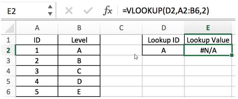
Example 2: Lookup value is incorrect; A is not listed in the first column of lookup table A2:B6.
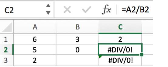
Error: #DIV/0!
Description: Function or formula has a divisor equal to 0 or the divisor cell is empty.
Solution: Change the divisor to a non-zero value.
Example:
Error: #NUM!
Explanation: A non-numeric value has been entered in the numeric argument or is out of Excel’s calculation range.
Solution: Check the argument type and enter a valid type.
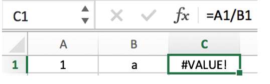
Error: #VALUE!
Explanation: Incorrect argument type entered, e.g., a number needs to be entered but text is entered, a value needs to be entered but multiple values are entered, etc. If it is an array formula, forget to press Control+Shift+Enter.
Solution: Check the argument type of the function and enter the correct type.
Example:
Divisor is “a”.
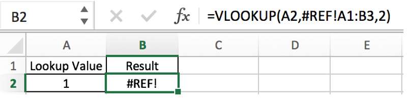
Error: #REF!
Explanation: Cell reference or range reference is invalid. For example, clear value in the cell reference which is used by the formula, then formula reports this error code.
Solution: make sure reference is correct; check if the cell reference or range reference is empty, and if it is, re-enter values into values.
Example:
Lookup table exists in sheet2, but sheet2 is deleted.
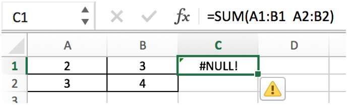
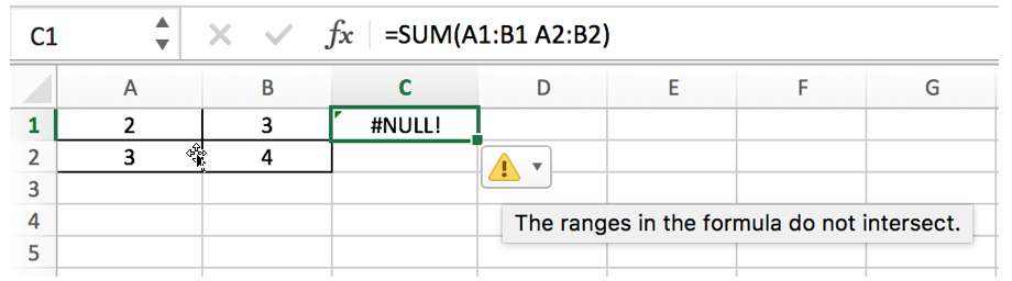
Error: #NULL!
Explanation: When multiple ranges are entered, the separator is incorrect; the intersection of multiple ranges is empty.
Solution: Change the separator; make the ranges intersect.
Example:
Separator is incorrect. It should be =SUM(A1:B1,A2:B2).
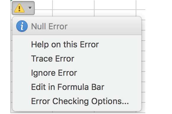
Resolution
We can move mouse over the warning icon to show the floating indication message.
You can also click the icon to do the following operations.
– Nested Functions
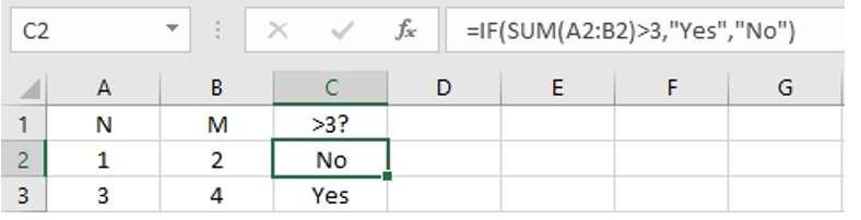
In addition to the arguments listed above, functions can also be used as arguments to a function, this is called nested function. The value of this internal function will be delivered to the external function as an argument value.
Example:
SUM(A2:B2)>3 is an argument (logical test) to IF function.
This article introduces some basic concepts in Excel or google sheets function applications, which are the most basis information for new learners. You can bookmark this article so that you can refer to it when learning functions or building formulas.