This post will guide you how to use 2 VLOOKUPS function to looking up data entries from a given range of cells in Microsoft Excel. VLOOKUP with 2 lookups can be faster than a single VLOOKUP in certain scenarios. The lookup times will, of course, depend on the data and the indexes.

The generic formula is as follow:

=IF(VLOOKUP(lookup_value,table_array,1,TRUE)=id, VLOOKUP(lookup_value,table_array,column_index,TRUE), NA())

Notes:

• This formula works very well if you have more than a few records. However, when speed really counts, use it with large data set.
• For this excel trick to work, you must sort the data by looking up a specific value.
• The following example uses absolute references. If you don’t want to use this, use named ranges instead!

Exact-match VLOOKUP Work Slow

---

Using the VLOOKUP function in “exact match mode” can be time-consuming when working with large data sets. For example, if you have 50 thousand or 100k records, it could take minutes just to do one lookup!

The exact match is determined by supplying FALSE or zero as the fourth argument:

=VLOOKUP(lookup_value,table_array,column_index,FALSE)

Using VLOOKUP in this mode will take forever because the program must check every single record until a match is found. This process of searching through all those data points can sometimes be referred to as linear search or even worst-case scenario: quadratic runtime!

Approximate-match VLOOKUP Works Efficiently and Quickly

---

Using the VLOOKUP function in “approximate match mode” is much more efficient when dealing with large data sets because it can quickly work through most of your records and return close-to-correct results.

Sometimes, this type of search is called a binary search since you search for approximate matches, not exact ones. The binary search is determined by supplying TRUE or 1 as the fourth argument:

=VLOOKUP(lookup_value,table_array,column_index,TRUE)

This simple change can literally speed up your worksheet calculations time by a factor of 100, where it would have taken minutes or hours to get a result with VLOOKUP.

The VLOOKUP function in “approximate match mode” can be faster than a single VLOOKUP because the program only needs to read and process half of your data at each iteration.

Problem with VLOOKUP Formula

---

VLOOKUP is a great tool for finding information in tables, but it can produce unexpected results when used without caution. For example, without using an exact match, VLOOKUP can return incorrect results when:

1. Data is sorted differently than the order of references in your formula, or data with similar-looking content is not sorted in the same way.
2. Your table has empty cells, and you did not anticipate this. Please see my previous article on VLOOKUP errors for more information on this topic.

These problems can be problematic when you need to get the exact information every time, especially when working with data sets that are either large or growing larger.

One way to avoid this is by doing two lookups to find an approximate match first and then verifying the result with an exact-match VLOOKUP.

Creating Formula to Perform 2 Lookups

---

This trick will work best when the key value sorts the data you are looking up, so using the same order in your formulas makes sense. The generic form of this formula is:

=IF(VLOOKUP(lookup_value,table_array,1,TRUE)=id, VLOOKUP(lookup_value,table_array,column_index,TRUE), NA())

This formula uses two lookups and will return “a match” when there is no. Another common alternative to using the last argument of False (exact match) for the first lookup is the Lookup_value argument instead.

Clarification

---

VLOOKUP is an incredible tool for finding exactly what you need. For instance, if I were looking up the value of STU ID in this example:

=VLOOKUP($F$2,$A$1:$C$12,1,TRUE)= $F$2

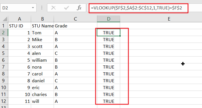
This looks up a value in an indexed array and returns TRUE only when the lookup is found. In that case, it uses VLOOKUP again with approximate match mode turned on to get you what’s left of your data:

VLOOKUP($F$2,$A$1:$C$12,2,TRUE)

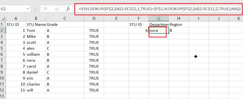
Or

VLOOKUP($F$2,$A$1:$C$12,3,TRUE)

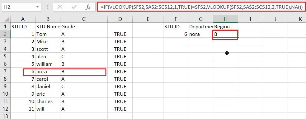
No need to worry about missing values since we have already checked the first part of this formula.

If the value isn’t found, then an error will be returned. For this example, we use NA(), which returns #N/A, but you could also return messages like ” Missing” or “Not Found”. This means that whatever value we put in place of “value” will be returned when it’s not found, such as “Missing” or Not Found.”

Related Functions

---

• Excel IF function
  The Excel IF function perform a logical test to return one value if the condition is TRUE and return another value if the condition is FALSE. The IF function is a build-in function in Microsoft Excel and it is categorized as a Logical Function.The syntax of the IF function is as below:= IF (condition, [true_value], [false_value])….
• Excel VLOOKUP function
  The Excel VLOOKUP function lookup a value in the first column of the table and return the value in the same row based on index_num position.The syntax of the VLOOKUP function is as below:= VLOOKUP (lookup_value, table_array, column_index_num,[range_lookup])….
• Excel NA function
  The Excel NA function returns the #N/A error value. And the #N/A is the error value that means “no values is available”. The syntax of the NA function is as below:= NA ( )….