Sometimes, the lookup value and the data table (containing the return value) are not in the same worksheet, or even in the same workbook. If you encounter a situation where the lookup value and the data table are stored in different worksheets, or in different workbooks, how does VLOOKUP handle this situation.

Lookup Value and Lookup Range in Same Worksheet

The simplest case is when the lookup value and the data table are in the same worksheet. This usually happens when there are not many lookup values, or when you are looking for a value temporarily. A common example is finding a value that corresponds to a value in the current data table. For example, finding an employee name or employee phone number based on an HRID.

See the following example.

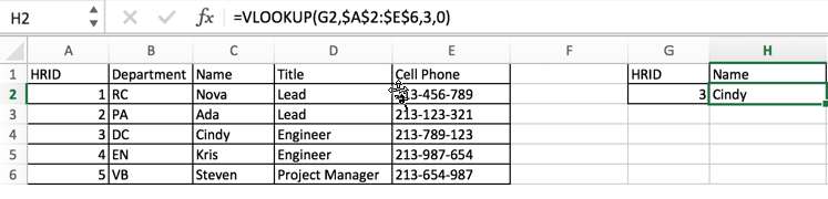
Formula:

=VLOOKUP(G2,$A$2:$E$6,3,0)

In this example, you can just operate the VLOOKUP function as usual. In the same worksheet, select the lookup value and lookup range, determine the column where the return value is located, and then select exact match or approximate match according to your needs, and you have completed a VLOOKUP lookup.

Arguments

Argument	Value	Description
lookup_value	G2	HRID=3
table_array	$A$2:$E$6	Locked range $A$2:$E$6
index_num	3	Return value in “Name” column
range_lookup	0	Exact match

Lookup Value and Lookup Range in Different Worksheets

Usually, the lookup value and lookup range (return value) may not be in the same worksheet. For example, in our daily work, due to user access rights settings, some information is saved in worksheet1, which can be opened by everyone, while some information is saved in worksheet2, which is only available to people with manager privileges. Only people who have access rights to both worksheets can open both worksheets for queries. At this point, when a manager wants to do an association of the two worksheets, they can use the VLOOKUP function to do a cross-sheet association.

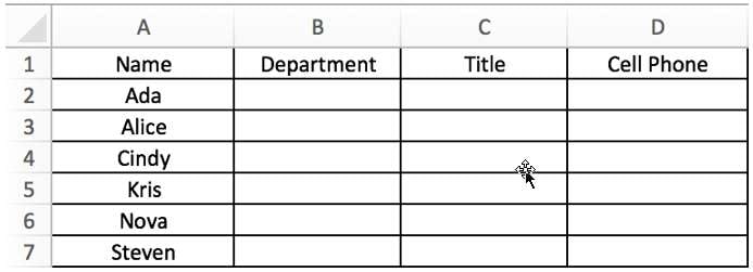
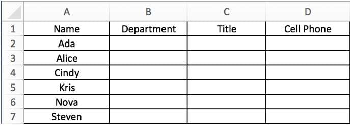
Sheet1 – A table with department, title, and cell phone information missing.

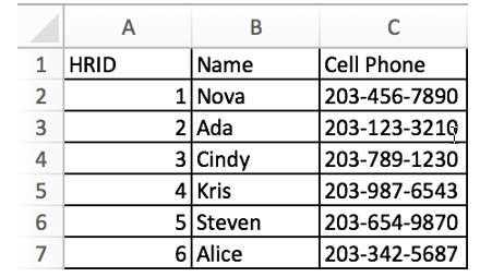
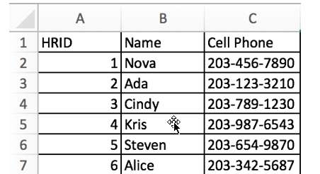
Sheet2 – Employee Personal Information

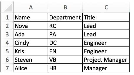
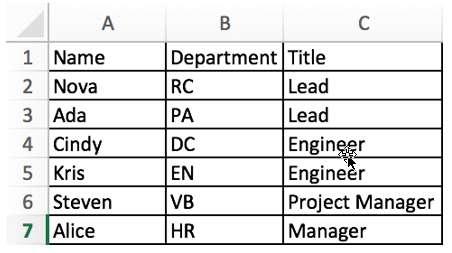
Sheet3 – Employee Function Information

To fill in the missing information in the first table, we need to use the name as a key to connect the tables in the other worksheets.

The steps are as follows.

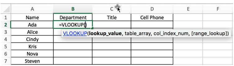
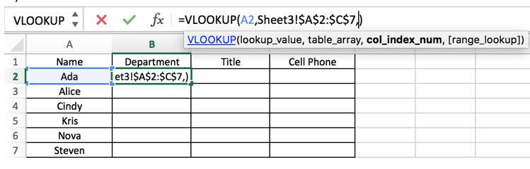
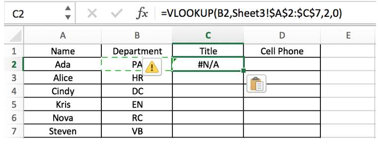
Step 1: In sheet1->B2, type “=VLOOKUP()”. A hint floats under “=VLOOKUP”.

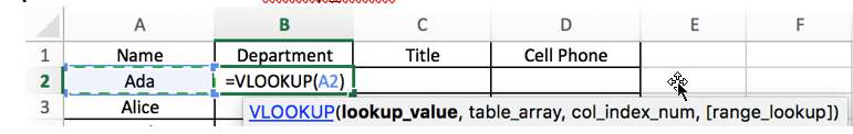
Step 2: Click A2 to fill in the lookup_value.

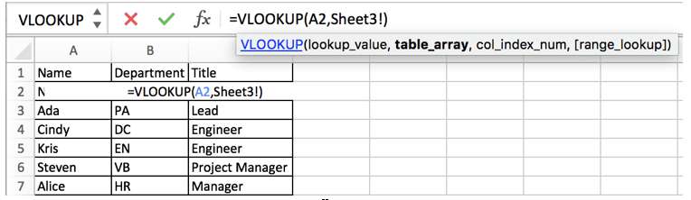
Step 3: Since department information is saved in sheet3, so we go to sheet3 and select the lookup range A2:C7.

Step 4: You will find that once you switch to sheet3, “Sheet3!” will be automatically filled into table_array.

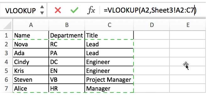
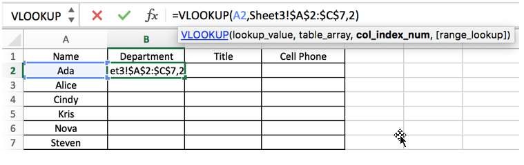
Step 5: Select lookup range A2:C7 to complete table_array.

Step 6: Add ($) to the formula to lock this range. Once ($) is entered before the column index, Excel will return to sheet1->B2.

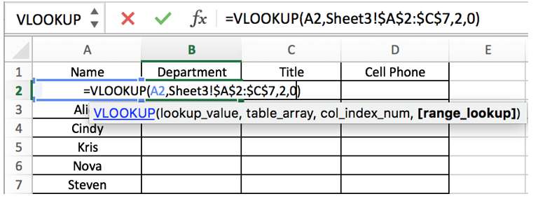
Step 7: Fill in col_index_num “2”. Department is the second list of lookup range.

Step 8: Enter “0” or “False”/ “1” or “True” to perform an exact match or an approximate match lookup.

Step 9: Press the Enter key to come up with a value.

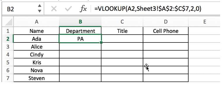
Step 10: Drag the handle down to fill the list. Because the lookup range is locked by ($), if you copy this formula to other cells, the lookup range will not be changed.

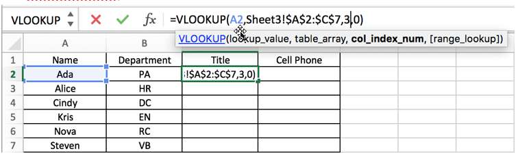
Step 11: Copy the formula from B2 to C2. The lookup value is changed to B2. Others are not changed.

Step 12: In the formula bar, update B2 to A2, keeping the query value unchanged. Update col_index_num to “3” because the title is saved in the third list of lookup range.

Step 13: Press the Enter key to come up with a value. Drag the handle down to fill the list.

Note: In this case, the department and title are saved in the same worksheet and they are adjacent to each other, we can create just one VLOOKUP formula to populate both lists at the same time. More details can be found in the section “VLOOKUP Returns Multiple Column Values”.

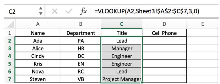
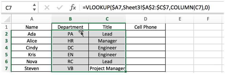
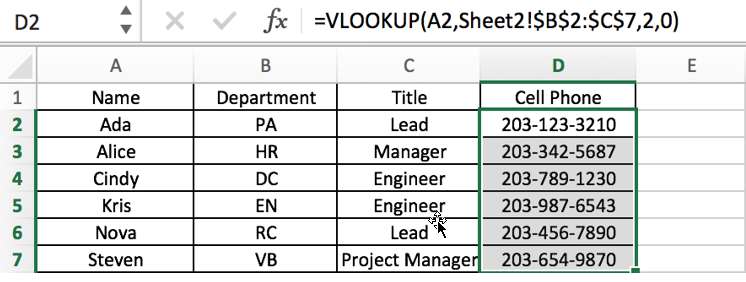
The formula is:

=VLOOKUP($A2,Sheet3!$A$2:$C$7,COLUMN(B2),0). 

Drag this handle to fill B2:C7.

Step 14: Repeat above steps to fill Cell Phone values.

Lookup Value and Lookup Range in Different Workbooks

We can see from the above example that when the lookup value and the lookup range are in two different Excel worksheets, the name of the worksheet where the lookup range is located will be added in front of the range reference, such as “Sheet2!$B$2:$C$7”. Therefore, the VLOOKUP function will go to the correct worksheet to look up the lookup value.

This time, we copy the data table from sheet1 to workbook 1->sheet A, then copy the table from sheet2 to workbook 2->sheet B, and then copy the table from sheet3 to workbook 3->sheet C. Now, the lookup values and lookup ranges are in three different workbooks rather than three different worksheets.

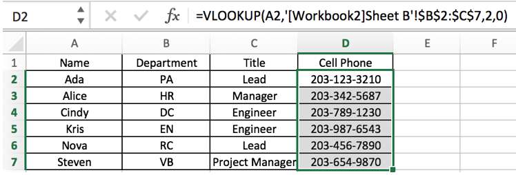
Workbook1->Sheet A

Workbook2->Sheet B

Workbook3->Sheet C

Now that workbook 1 lists a table with employee names, departments and cell phone numbers, we want to populate the other employee information based on the first column of employee names. The other information is saved in workbook 2 and workbook 3 respectively. Since the name is the only value that appears in these three tables, it can be associated with all three workbooks.

The steps are as follows.

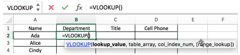
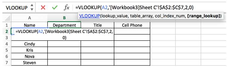
Step 1: In workbook1->sheet2->B2, type “=VLOOKUP()“. A hint floats under “=VLOOKUP“.

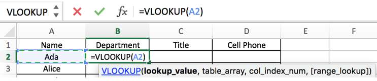
Step 2: Click A2 to fill in the lookup_value.

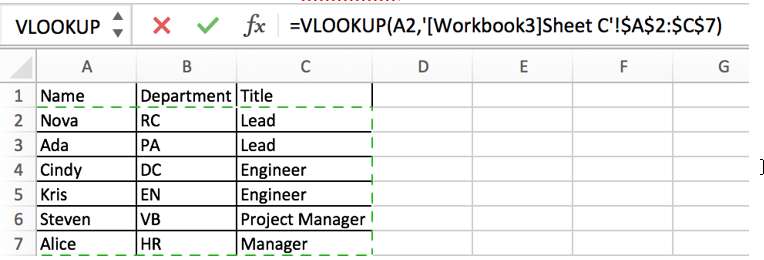
Step 3: Since department information is saved in workbook3->sheet C, so we go to orkbook3->sheet C to select the lookup range A2:C7.

Step 4: Go to workbook3->sheet C. You will find that once you switch to sheet C.

‘[Workbook3]Sheet C’! will be automatically filled into table_array. Select the lookup range A2:C7 to complete the filling of table_array. the range is automatically locked.

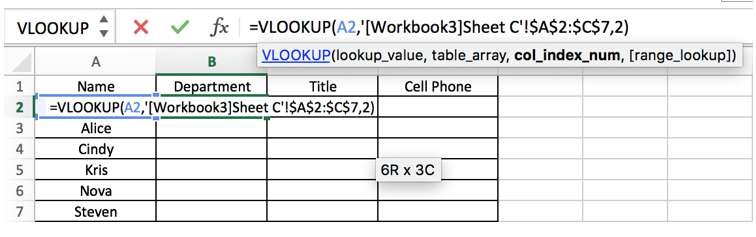
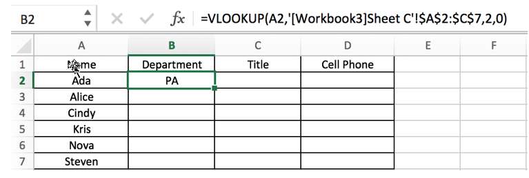
Step 5: Return to workbook1->Sheet A. Fill in col_index_num “2”. Department is the second list of lookup range.

Step 6: Enter “0” or “False”/ “1” or “True” to perform an exact match or an approximate match lookup.

Step 7: Press the Enter key to come up with a value.

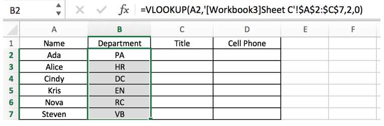
Step 8: Drag the handle down to fill the list. Because the lookup range is locked by ($), if you copy this formula to other cells, the lookup range will not be changed.

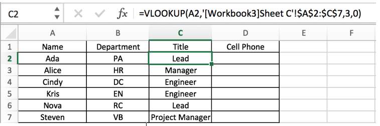
Step 9: Copy the formula from B2 to C2. The lookup value is changed to B2. Others are not changed. Update B2 to A2, keeping the lookup value unchanged. Update col_index_num to “3” because the title is saved in the third list of lookup range.

Note:

In this case, the department and title are saved in the same worksheet and they are adjacent to each other, we can create just one VLOOKUP formula to populate both lists at the same time. More details can be found in the section “VLOOKUP Returns Multiple Column Values”.

The formula is:

 =VLOOKUP($A2,'[Workbook3]Sheet C'!$A$2:$C$7,COLUMN(B1),0). 

Drag this handle to fill B2:C7.

Step 10: Repeat above steps to fill Cell Phone values.