This article will talk about how to rank the given data in reverse order in google sheets. You can use Google sheets RANK function to rank the data. By default, the largest value in the data table will be ranked as 1. So how do we invert this ranking order? How do we make the smallest value ranked as 1? So how do we achieve this requirement?
Table of Contents
Reverse Rank Order
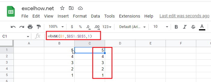
Suppose you have a list of data and you want to sort these data and later reverse the sort order on them? If you do the ranking by manually, it is definitely not a good way to handle it. The best way is to use the RANK function to sort the data. To reverse the sort order, you just need to add a new parameter to the RANK function. The formula is as follows.
=RANK(B1,$B$1:$B$5,1)
As you can see from the above example, the sorting result has been reversed.

Related Functions
- Google Sheets RANK Function
The Google Sheets Rank function is used to return the ranking of a given number from a list. If there are duplicate numbers in the list, then the numbers will be in the same rank.The syntax of the Google Sheets Rank function is explained as follows:The syntax of the Google Sheets Rank function is explained as follows:= RANK (number,reference ,[order])…