This post will guide you how to rank data in reverse order in Excel. You can use the RANK function to rank data in excel, and the biggest value will be ranked as 1 by default. How to reverse this rank order and lets the smallest value be ranked as 1. How to achieve it in excel.
Table of Contents
Reverse Rank Order
Assuming that you have a formula based on RANK function that ranks numbers by biggest to smallest by default. But you want to go the opposite from the smallest to biggest. So you need to reverse the rank order to achieve it.
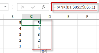
To reverse rank order in excel, you just need to add one more argument in the Rank function, just like this formula:
=RANK(B1,$B$1:$B$B5,1)

You will see that the rank order has been reversed.
Related Functions
- Excel Rank function
The Excel RANK function returns the rank of a given number in a supplied range of cells. If there are duplicated values in a list of values, it will be set the same rank.The syntax of the RANK function is as below:= RANK (number,ref,[order])….
Leave a Reply
You must be logged in to post a comment.