VLOOKUP function is extremely strong among excel all functions and it is very useful in our daily work. It can save a lot of time if we want to find matching value from a long list and return the value we want. Normally we can find exact or approximate matching value from a list by setting False of True (the last argument) in formula =VLOOKUP(lookup_value, table_array, col_index_num, [range_lookup]). If there is only one matching value, we can find it out easily no matter we set False or Ture to get exact or approximate matching value. But if there are more than one matching value, which matching value will be found? The first one or the last one? Actually, if we set False to get exact matching value, the first matching value will be found. On the other side, if we set True, the last matching value will be found instead. This article will show you some examples, now let’s see them.
Precondition:
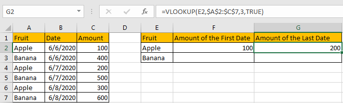
Prepare two tables. In table1 we list different amounts for apple and banana on different dates. In table2 we list the amount for apple and banana on the first date and the last date. Obviously, we can use VLOOKUP function here to find matching value in Fruit column and then return amount value in Amount column. For “Amount of the First Date”, we can use VLOOKUP function to find the first matching value, for “Amount of the Last Date”, we can find the last matching value. Now let’s see steps below for finding first and last matching value.
Table 1:
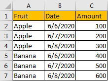
Table 2:
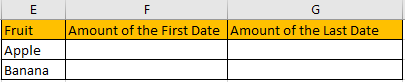
Table of Contents
Part 1: Use VLOOKUP to Find the First Matching Value
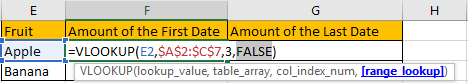
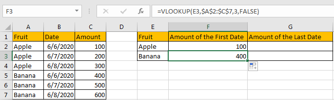
Step 1: In F2, enter the formula =VLOOKUP(E2,$A$2:$C$7,3,FALSE). Notice that we set range_lookup to False to get exact matching value here.
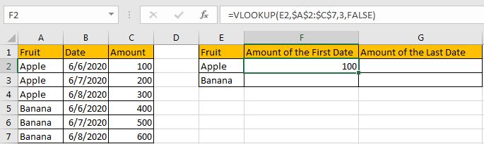
Step 2: Click Enter to get returned value. Verify that the first matching value is found in this case.
Step 3: Drag cell F2 down with formula to fill cell F3.
Now we can make sure that if there are more than one matching value exist in the list, we can set range_lookup to False to find the first matching value.
Part 2: Use VLOOKUP to Find the Last Matching Value
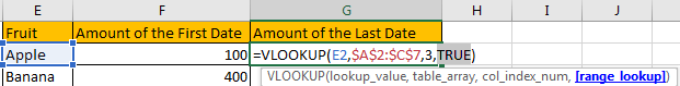
Step 1: In G2, enter the formula =VLOOKUP(E2,$A$2:$C$7,3,TRUE). Notice that we set range_lookup to True to get approximate matching value here.
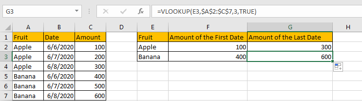
Step 2: Click Enter to get returned value. Verify that the last matching value is found in this case.

Step 3: Drag cell G2 down with formula to fill cell G3. Verify that we get the last matching value properly.
Comment:
In above example, the matching values are sorted properly. If they are not sorted, we may get improper value with above formula. See table below.
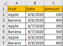
In G2, we still enter the formula =VLOOKUP(E2,$A$2:$C$7,3,TRUE).After clicking Enter, we get 200, which is the amount for the second Apple in list.
So please be aware that if we want to get last matching value by setting True in formula, we must make sure the matching values are sorted properly.
Related Functions
- Excel VLOOKUP function
The Excel VLOOKUP function lookup a value in the first column of the table and return the value in the same row based on index_num position.The syntax of the VLOOKUP function is as below:= VLOOKUP (lookup_value, table_array, column_index_num,[range_lookup])….