This post will guide you how to use VLOOKUP function to look up values based on an exact or approximate match in Excel 2013/2016 or the higher versions. VLOOKUP function can search a range of cells for a specific value or data and if a match is found, and it will return a piece of data from that matching.
In most of cases, you can be use VLOOKUP function to find exact matches from a given range of cells based on some kind of value in your worksheet. Also you can also use VLOOKUP function to find non-exact or approximate matches to achieve your request.
If you still do not know what is exact or approximate matches in VLOOKUP function in Microsoft Excel, and it is recommend to have a quick look of my earlier post on how to use Excel Vlookup function.
Assuming that you have a sales data in cell Range A1:C6, and you want to find a sales number based on a product id, and you can use the following vlookup formula into a blank cell where you can to show the result.
Table of Contents
1. Use of VLOOKUP function to Extract Approximate Matches
If you want to calculate the discount based on the quantity sold in your worksheet, and assuming that you want to search a sales number 60 to calculate its discount value, which doesn’t exist in your data A1:D6. And to search for an approximate matches based on your specified sales number 60, just type the following VLOOKUP formula into cell G2.
=VLOOKUP(F2,C1:D6,2,TRUE)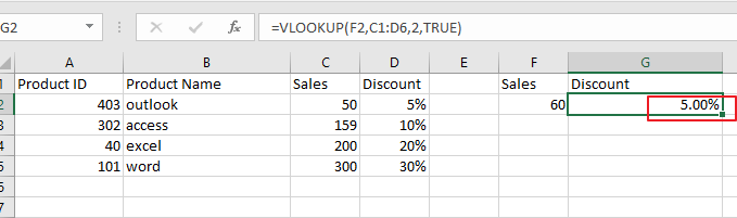
Note: the Cell F2 is the searched value which you want to get it the appropriate discount number. C1:D6 is the data range that you are using. The number 2 is that your matched value is returned. The TRUE value indicates that you want to calculate the approximate match.
Before applying the above formula, you need to make sure that your sales column is sorted in ascending order. Or the VLOOKUP formulas stop working properly and you will get a N/A errors.
2. Use of VLOOKUP function to get Exact Matches
Now let’s add this VLOOKUP formula in cell G2 to calculate the appropriate sales number based on the product id in cell F2.
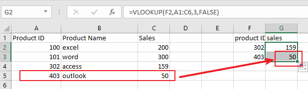
=VLOOKUP(F2,A1:C6,3,FALSE)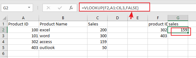
If you wish to search for multiple values in the same column, and you just need to drag the fill handle (G2) down to other cells to apply this formula.
Note: you need to set a value for range_lookup argument, and it is set to FALSE or 0, VLOOKUP will find a exact match. And if it is set to 1 or TRUE, VLOOKUP will search for the closest match.
3. Video: Use VLOOKUP for Approximate or Exact Matches
This Excel video tutorial, we’re going to learn how to use the V LOOKUP function to find both approximate and exact matches.
4. Related Functions
- Excel VLOOKUP function
The Excel VLOOKUP function lookup a value in the first column of the table and return the value in the same row based on index_num position.The syntax of the VLOOKUP function is as below:= VLOOKUP (lookup_value, table_array, column_index_num,[range_lookup])….