Create a Pivot Table | Refresh a Pivot Table | Filter a Pivot Table | Change data source for pivot table | Remove column/row Grand Totals | Change pivot table name | Sort pivot table results | Change the type of calculation | Two-dimensional Pivot table

A Pivot Table allows you to extract certain data from a much larger data set to summarize complex data. This post will guide you how to use pivot table in Microsoft excel from the below subjects:

• Create a Pivot Table
• Refresh a Pivot Table
• Filter a Pivot Table
• Change data source for pivot table
• Remove column/row Grand Totals
• Change pivot table name
• Sort pivot table results
• Change the type of calculation
• Two-dimensional Pivot table

Create a Pivot Table

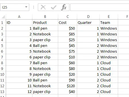
The below data set will be used in the following pivot table examples.

To create a new Pivot table, just follow the below steps:

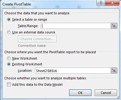
#1 Click any single cell in which you want to insert pivot table (select B16 in this example).

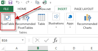
#2 Click “INSERT” in the Ribbon tab, then clicking “Pivot Table” button in the “Tables” group.

#3 A “Create PivotTable” window will appear.

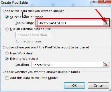
#4 Select a range “A1:E13” for the pivot table and click on the OK.

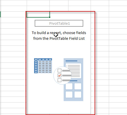
#5 A Pivot Table will appear and “Pivot Table Fields” Layout also will appear in the right of window.

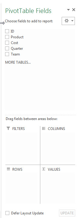
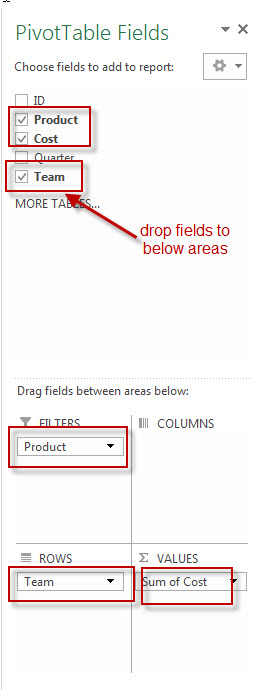
#6 Drag “Product” field to the Filters area, “Team” field to the Row area and “Cost” field to the Values area.

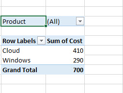
Now the PivotTable report is generated as follows:

Refresh a Pivot Table

If the data source make some changes, then you need to refresh your pivot table to take effect. To refresh pivot table, just following the below steps:

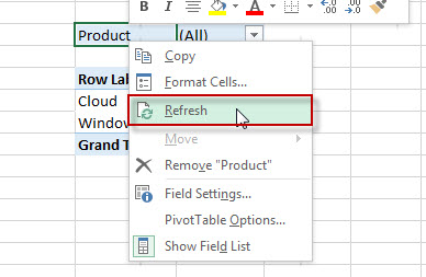
1# right-click on the pivot table, then click “refresh”

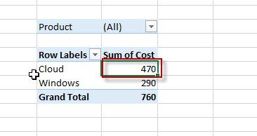
2# You will see that the pivot table refreshed. The sum of cost value have been changed from 410  to 470.

Filter a Pivot Table

When creating pivot table, we need to drag fields to the Filters area, so we can filter this pivot table by this field that you dragged. In the above example, the “Product” field is dragged to the Filters area, so we can filter this pivot table by “Product” field. Just following the below steps:

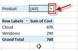
#1 Click the filter drop-down button

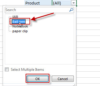
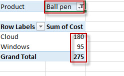
#2 select one item from the drop-down list. Such as: select “Ball pen”. Then click “OK” button.

#3 let’s see the filter result.

Change data source for pivot table

After created a PivotTable, you can change the range of its source data, such as, you can expand the source data to include more rows of data.

To change the data source for pivot table, just following the below steps:

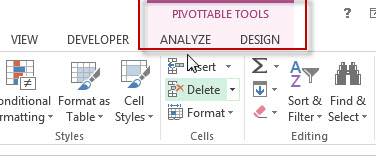
#1 click any cell inside the pivot table, then the “PivotTable Tools” tab will show on the ribbon.

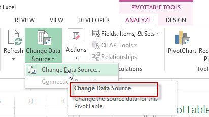
#2 click “ANALYZE” Tab, then click “Change Data Source”.

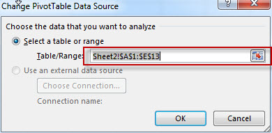
#3 the window of “Change PivotTable Data Source” will appear, then enter the range that you want to use.

Remove column/row Grand Totals

If you want to remove grand totals for columns, just do the following:

#1 click “DESIGN” Tab under “PivotTable Tools” in Ribbon.

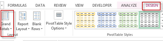
#2 click “Grand Totals” button and then select “On for Rows Only”.

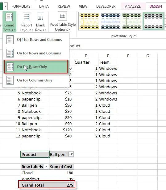
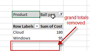
#3 let’s see the result:

Change pivot table name

By default, the first pivot table you create is named as “PivotTable1”, the second is “PivotTable2”… so on.  The below steps will guide you how to rename the existing pivot table, just do the following:

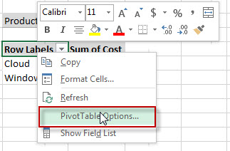
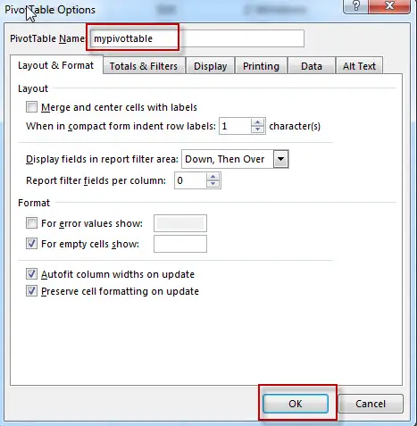
#1 Right click any cell inside the pivot table and then select “PivotTable Options”

#2 enter into the pivot table name that you want to use in the “PivotTable Name” textbox. Then click “OK” button.

Sort pivot table results

To sort the pivot table result, just following the below steps:

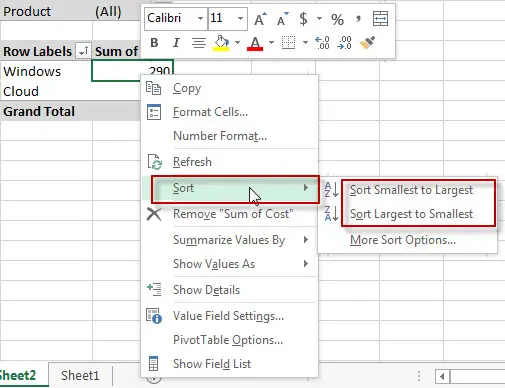
#1 right click any cell inside the “sum of Cost” field in the pivot table.

#2 click “Sort”, then click “sort Largest to Smallest” or “sort Smallest to Largest” from the popup menu

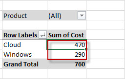
#3 the results of “sum of Cost” will be sort.

Change the type of calculation

By default, Excel will summarizes value field by summing the items. To change the type of calculation that you want to use to summarize data from the selected field, just following the below steps:

#1 click any cell inside the “Sum of Cost” column, then click “Value Field Settings…”

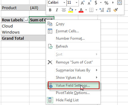
#2 the window of “Value Field Settings” will appear.

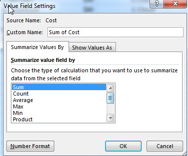
#3 choose one type of calculation you want to use under “Summarize Values By” Tab. Then click OK button.

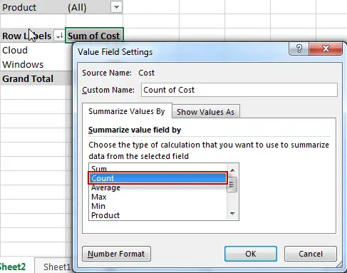
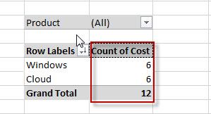
#4 let’s see the result:

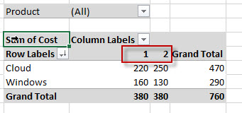
Two-dimensional Pivot table

Two-dimensional Pivot table can be created by dragging a field to the Rows area and Columns area.  The following steps will guide you how to create a two dimensional pivot table:

#1 insert a pivot table, then drag “Product” field to the Filters area, “Team” field to the Row area, “Quarter” field to the Columns area and “Cost” field to the Values area in the “PivotTable Fields” dashboard.

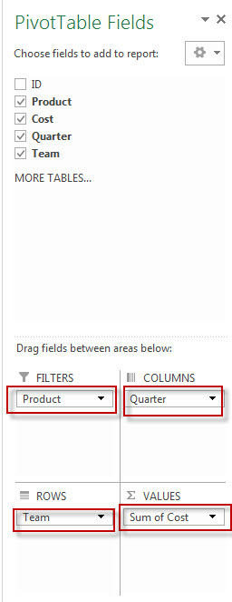
#2 let’s see the result: