If we want to add numbers based on some conditions in Excel worksheet, we can add criteria with the help of SUMIFS function, SUMIFS can filter data with multiple criteria effectively. In this article, we will introduce you the method about applying SUMIFS function to sum numbers with different vertical ranges.
We will introduce you the syntax, arguments of SUMIFS function, and let you know how this formula works to reach your goal. After reading the article, you may have a simple understanding of SUMIFS function and know how can we use this function to sum numbers with vertical range.
Table of Contents
1. Sum in Vertical Range Example
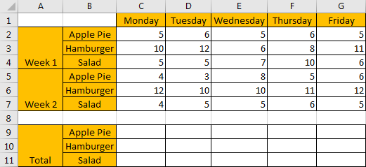
Refer to the upper side table, it lists the amount for ‘Apple Pie’, ‘Hamburger’ and ‘Salad’ on weekdays (from ‘Monday’ to ‘Friday’) in two weeks. Start from column C, it lists the amount for the three kinds of food on each weekday for two weeks in vertical direction. In the bottom side table, it records the total amount for the three kinds of food in two weeks.
Now, we need to create a formula that can return the total amount for each food in two weeks based on different weekdays. This question can be seen as we need to sum data from a vertical range with specific criteria. For example, in this instance, in C9, we want to enter a formula that can return the total amount for ‘Apple Pie’ on ‘Monday’ in ‘two weeks’ (week1 and week2). Besides, when dragging the formula to other cells (in range reference C9 to G11), we need the formula can adjust cell reference and range reference automatically and return the correct result based on updated parameters properly.
In this instance, we need to pick up numbers with criteria from each vertical range, then sum them together. To fix this issue by formula, we can apply excel built-in function SUMIFS here.
2. Sum in Vertical Range Formula – SUMIFS FUNCTIONS
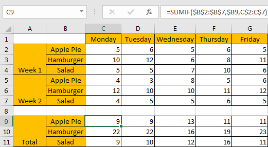
Step1: In C9, enter the formula
=SUMIFS(C$2:C$7,$B$2:$B$7,$B9)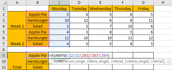
Step2: Press Enter after typing the formula.
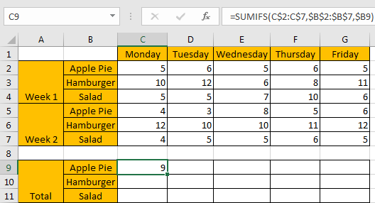
We can see in cell C9 result 9 is returned, it is equal to 5 from C2 plus 4 from C4, the formula works correctly.
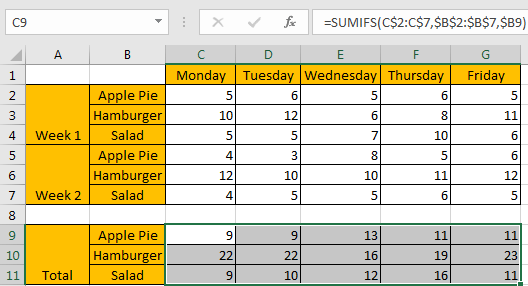
Step3: Drag the ‘Auto Fill’ handle to make range reference C9:G11 filled with the formula. Then we can see that results are automatically calculated and displayed in each cell correctly.
3. SUMIFS FUNCTION INTRODUCTION
SUMIFS function can be seen as SUM+IFS, it can handle multiple ‘criteria range’ and ‘criteria’ combinations.
Syntax:
=SUMIFS(sum_range, criteria_range1, criteria1, [criteria_range2, criteria2], ...)[] part can be omitted.
For SUMIFS function, it supports wildcards like asterisk ‘*’ and question mark ‘?’, also support logical operators. If wildcards or logical operators are required, they should be enclosed into double quotes (““).
The usage of wildcards:
- An asterisk (*) means one or more characters.
- A question mark (?) means one character.
- The position of asterisk or question mark means the character(s) position relative to the entered part.
The usage of logical operators:
- “>” – greater than
- “<” – less than
- “<>” – not equal to
ALL ARGUMENTS
The formula is =SUMIFS(C$2:C$7,$B$2:$B$7,$B9). Refer to above SUMIFS function introduction, we will split it to several parts.
SUMIFS – SUM RANGE
C$2:C$7 is the ‘sum range’ in this case.
You can see we add “$” before row index 2 and 7, that’s because when dragging the formula from C9 to C10 (formula is moved in vertical direction), cell reference will be moved in vertical direction by default, so we need add “$” before row index to lock the range in vertical direction, make sure the sum range can only be adjusted in vertical, but in horizontal, it is absolutely fixed.
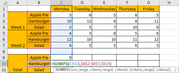
See screenshot below, if “$” is omitted, formula is updated to =SUMIFS(C3:C8,$B$2:$B$7,$B10) in C10, sum range is moved from range reference C2:C7 to C3:C8 improperly, the returned result is 9 incorrectly.
Select C$2:C$7 from formula in the formula bar, the press F9, values in this range are expanded in an array.
SUMIFS – CRITERIA RANGE
$B$2:$B$7 is the criteria range. We have only one criteria range in this instance.
Criteria range contains three kinds of food, due to there are two weeks, so we list them twice.
You can see we add “$” before column and row index both, that’s because range $B$2:$B$7 is an absolute range. No matter copy formula to which cell reference, the criteria range is still $B$2:$B$7 and will not be changed. So we add ‘$’ to lock this range.
Select $B$2:$B$7 from formula in the formula bar, the press F9, values in this range are expanded in an array.

SUMIFS – CRITERIA
$B9 is the criteria. $B9=”Apple Pie”.
As we want to calculate total amount for the provided food, so can set criteria as B9 (B9=”Apple Pie”), B10 (B10=”Hamburger”), and B11 (B11=”Salad”). As column B is fixed, so we add ‘$’ before column B.
We can also enter food name directly, as SUMIFS function supports texts, but they should be enclosed into double quotes “”, so for criteria “Apple Pie”, we can directly enter “Apple Pie” in criteria argument.
Select $B9 from formula in the formula bar, the press F9, criteria value is displayed.

4. Sum in Vertical Range – Formula Explantation
After explaining each argument in the formula, now we will show you how the formula works with these arguments.
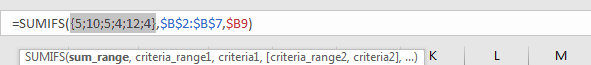
After expanding values in each range reference or cell reference, in the formula bar, the formula is displayed as:
=SUMIFS({5;10;5;4;12;4},{"Apple Pie";"Hamburger";"Salad";"Apple Pie";"Hamburger";"Salad"},"Apple Pie")There is one pair of criteria range and criteria.
{“Apple Pie”;”Hamburger”;”Salad”;”Apple Pie”;”Hamburger”;”Salad”} – Criteria Range
{“Apple Pie”} – Criteria
If values from the criteria range are matched with the criteria “Apple Pie”, “True” will be recorded and saved, otherwise, “False” will be saved instead. So, after comparing, we can get a new array:
{True;False;False;True;False;False} – after comparing with criteria “Apple Pie”
For the following logical operation, “True” is coerced to ‘1’ and ‘False’ is coerced to ‘0’. So above array is converted to below array which consists of numbers “1” and “0”.
{1;0;0;1;0;0} – for criteria “Apple Pie”
Now, we have below two pairs of arrays:
{5;10;5;4;12;4} – sum range
{1;0;0;1;0;0} – for criteria “Apple Pie”
Multiply the two elements in the same position in the two arrays. Then we can get a new array.
{5;0;0;4;0;0}
Add all products in above array, we get 9 finally. Actually, in step#2, SUMIFS function returns 9 after calculation. For the other cells, the workflow is similar.
COMMENTS
1. In this case, as we have only one pair of criteria range and criteria, we can also apply SUMIF function as well. The difference is SUMIF function only supports one group of criteria range and criteria, and its sum range is listed at the end.
Enter =SUMIF($B$2:$B$7,$B9,C$2:C$7), we can get the same result as applying SUMIFS.
5. Video: How to Sum in Vertical Range in Excel
In this video, you will learn how to use the SUMIF formula to sum values in a vertical range in Excel.
6. Related Functions
- Excel SUMIF Function
The Excel SUMIF function sum the numbers in the range of cells that meet a single criteria that you specify. The syntax of the SUMIF function is as below:=SUMIF (range, criteria, [sum_range])… - Excel SUMIFS Function
The Excel SUMIFS function sum the numbers in the range of cells that meet a single or multiple criteria that you specify. The syntax of the SUMIFS function is as below:=SUMIFS (sum_range, criteria_range1, criteria1, [criteria_range2, criteria2], …)… - Excel SUM function
The Excel SUM function will adds all numbers in a range of cells and returns the sum of these values. You can add individual values, cell references or ranges in excel.The syntax of the SUM function is as below:= SUM(number1,[number2],…)