To add numbers together we need to apply SUM function. And if we want to add numbers based on some conditions, we can add criteria with the help of SUMIFS function, SUMIFS can filter data with multiple criteria effectively. If we want to sum cells with special character only, for example sum cells which contains an asterisk “*”, we can use “*~**” to represent the cells. In this article, we will introduce you the syntax, arguments of SUM and SUMIFS function, and why we use “*~**” to stands for the selected items. We will also let you know how the formula works step by step. After reading the article, you may have a simple understanding about SUMIFS function and the usage of asterisk (*).
Table of Contents
EXAMPLE
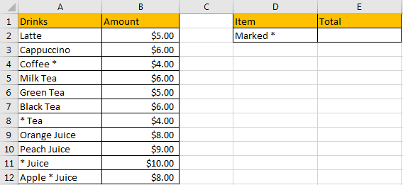
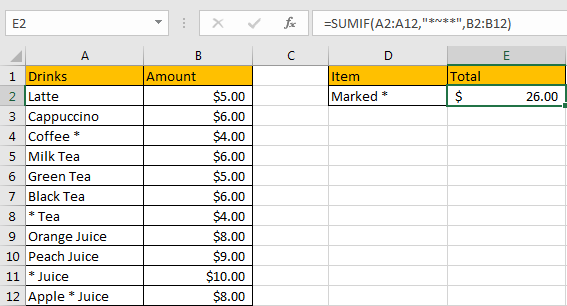
Refer to the left-hand side table, we can see some kinds of drinks and their amounts are listed. Some items are marked with an asterisk (*) in its name for example “Coffee *”, it represents an unknow type of coffee or any coffee is ok. In the right-hand side table, in “Item” column, we can list the kind of drink we want, and in the “Total” column, total amount will be calculated and listed in E2 properly based on the selected items. We need to enter a formula into E2 to calculate total amount automatically. In this case, the items are that marked with an asterisk, now we need to create a formula that can calculate all amounts for those drinks marked with an asterisk. To create a formula, we can apply SUMIFS function here.
FORMULA – SUM & SUMIFS FUNCTIONS
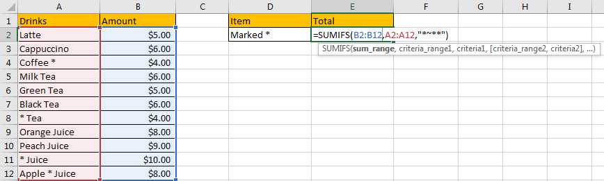
Step 1: In E2, enter the formula
=SUMIFS(B2:B12,A2:A12,"*~**").
Step 2: Press Enter after typing the formula.
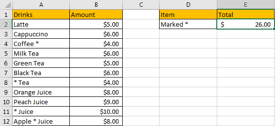
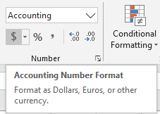
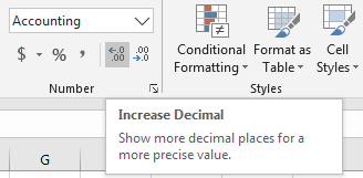
We can see $26.00 is returned. The format is correct. Actually, if you didn’t set the format for cell E2 before, only “26” is returned. Before entering the formula, you need to focus on this cell, and click ‘Dollars’ icon under ‘Number’ section, and also double click on ‘Increase Decimal’ icon to add two decimal places for the returned number.
Now, let’s check the result. in column A, cell A4, A8, A11 and A12 meet our demand, so we just need to sum amounts from B4, B8, B11 and B12, so the total number is 4+4+10+8=26. The formula works correctly.
FUNCTION INTRODUCTION
SUMIFS function can be seen as SUM+IFS, it can handle multiple ‘criteria range’ and ‘criteria’ combinations.
Syntax:
=SUMIFS(sum_range, criteria_range1, criteria1, [criteria_range2, criteria2], ...)
[] part can be omitted.
For SUMIFS function, is supports wildcards like asterisk ‘*’ and question mark ‘?’, also support logical operators like “>”,”<”. If wildcards or logical operators are required, they should be enclosed into double quotes (““).
The usage of wildcards:
- An asterisk (*) means one or more characters.
- A question mark (?) means one character.
- The position of asterisk or question mark means the character(s) position relative to the entered part.
The usage of logical operators:
- “>” – greater than
- “<” – less than
- “<>” – not equal to
Notes:
In this case, as an asterisk stands for one or more characters by itself, so we need to add a “~” before it to make it only stands for special character “*” literally, then Excel can handle it properly and treat it as an asterisk in formula working process. As there might be some other characters before or after special character “*” in items, so we need to add “*” before and after “~*”. Finally, to represent an item contains an asterisk, we use “*~**” to stand for it.
ALL ARGUMENTS
The formula is =SUMIFS(B2:B12,A2:A12,”*~**”). Refer to above SUMIFS function introduction, we will split it to several parts.
SUMIFS – SUM RANGE
B2:B12 is the ‘sum range’ in this case.
Select B2:B12 from formula in the formula bar, the press F9, values in this range are expanded in an array.
SUMIFS – CRITERIA RANGE
A2:A12 is the criteria range. We have only one criteria range in this instance.
Criteria range contains some kinds of drinks, some of them contain an asterisk, we need to pick them up.
Select A2:A12 from formula in the formula bar, the press F9, values in this range are expanded in an array.

SUMIFS – CRITERIA
D2 is the criteria. D2=”*~**”.
As we mentioned before, “~*” can stand for a literal asterisk. “*~**” stands for items that contain one asterisk. If characters are only listed before the asterisk, you can also set “*~*” as criteria.
HOW THE FORMULA WORKS
After explaining each argument in the formula, now we will show you how the formula works with these arguments.
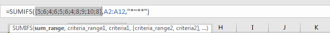
After expanding values in each range reference, in the formula bar, the formula is displayed as:
=SUMIFS({5;6;4;6;5;6;4;8;9;10;8},{"Latte";"Cappuccino";"Coffee *";"Milk Tea";"Green Tea";"Black Tea";"* Tea";"Orange Juice";"Peach Juice";"* Juice";"Apple * Juice"},"*~**")
There is one pair of criteria range and criteria.
{"Latte";"Cappuccino";"Coffee *";"Milk Tea";"Green Tea";"Black Tea";"* Tea";"Orange Juice";"Peach Juice";"* Juice";"Apple * Juice"} – Criteria Range
{“*~**”} – Criteria
If values from the criteria range are matched with the criteria “marked with an asterisk”, “True” will be recorded and saved, otherwise, “False” will be saved instead. So, after comparing, we can get a new array:
{False;False;True;False;False;False;True;False;False;True;True}
– after comparing with criteria
For the following logical operation, “True” is coerced to ‘1’ and ‘False’ is coerced to ‘0’. So above array is converted to below array which consists of numbers “1” and “0”.
{0;0;1;0;0;0;1;0;0;1;1} – criteria range “1” means which can meet the criteria
Now, we have below two arrays:
{5;6;4;6;5;6;4;8;9;10;8} – sum range
{0;0;1;0;0;0;1;0;0;1;1} – criteria range
Elements are horizontal-aligned in the two arrays. Multiply the two elements in the same position in the array. Then we can get a new array.
{0;0;4;0;0;0;4;0;0;10;8}
Add all products in above array, we get 26.
COMMENTS
1.In this case, as we have only one pair of criteria range and criteria, we can also apply SUMIF function as well. The difference is SUMIF function only supports one group of criteria range and criteria, and its sum range is listed at the end.
Enter =SUMIF(A2:A12,”*~**”,B2:B12), we can get the same result as applying SUMIFS.
Sum if Contains an Asterisk using VBA with User-Defined Function
Now, let’s embark on our VBA journey with the second method—a user-defined function crafted for summing values with asterisks.
Press Alt + F11 to open the Visual Basic for Applications (VBA) editor.
In the editor, go to Insert > Module to add a new module.
Copy and paste the provided VBA code into the module.
Function SumIfContainsAsterisk(rngCriteria As Range, rngValues As Range) As Double
    Dim i As Long
    Dim sumResult As Double

    ' Loop through each cell in the criteria range
    For i = 1 To rngCriteria.Rows.Count
        ' Check if the cell contains an asterisk
        If InStr(1, rngCriteria.Cells(i, 1).Value, "*") > 0 Then
            ' If true, add the corresponding value to the sum
            sumResult = sumResult + rngValues.Cells(i, 1).Value
        End If
    Next i

    ' Return the final sum
    SumIfContainsAsterisk = sumResult
End Function
Close the VBA editor.
Return to your Excel workbook.
In a cell where you want the result, type the following formula:
=SumIfContainsAsterisk(A2:A12, B2:B12)Press Enter, and the corrected VBA function will sum values in column B corresponding to cells in column A that contain an asterisk.
Video: Sum if Contains an Asterisk
This Excel video tutorial, where we’ll tackle the challenge of summing values containing an asterisk. In this exploration, we’ll employ two robust methods to achieve our goal—a formulaic solution within Excel and a VBA-driven user-defined function.
Related Functions
- Excel SUMIF Function
The Excel SUMIF function sum the numbers in the range of cells that meet a single criteria that you specify. The syntax of the SUMIF function is as below:=SUMIF (range, criteria, [sum_range])… - Excel SUMIFS Function
The Excel SUMIFS function sum the numbers in the range of cells that meet a single or multiple criteria that you specify. The syntax of the SUMIFS function is as below:=SUMIFS (sum_range, criteria_range1, criteria1, [criteria_range2, criteria2], …)… - Excel SUM function
The Excel SUM function will adds all numbers in a range of cells and returns the sum of these values. You can add individual values, cell references or ranges in excel.The syntax of the SUM function is as below:= SUM(number1,[number2],…)