In our daily life, we may want to sum amounts or sales for a specific period, for example in last N days. Sum numbers in Excel is easy to run, we can apply SUM function. But if we want to sum numbers based on criteria, we can SUMIF or SUMIFS function, compare with SUMIF function, SUMIFS can handle multiple criteria effectively.
In this article, we will provide a simple case to show you the way we use SUMIFS function to sum amounts for different items in last 3 days. We will introduce you the syntax, arguments of SUMIFS function, create a formula to sum numbers per our demand. We will also split the formula to several parts and let you know how the formula works step by step. After reading the article, you may have a simple understanding about SUMIFS function and you can use it to sum in last n days.
Table of Contents
EXAMPLE
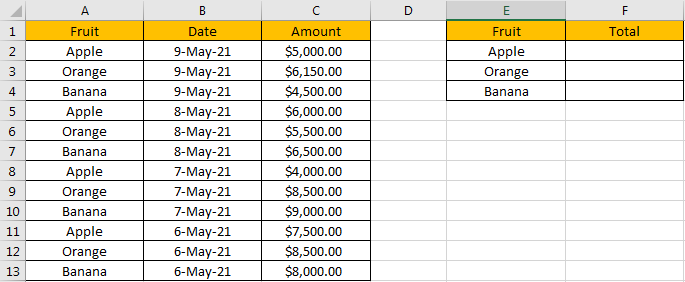
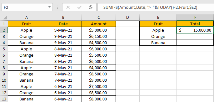
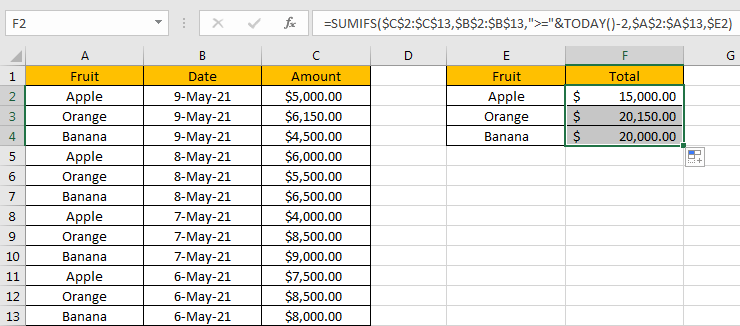
Refer to the left-hand side table, we can see some kinds of fruits and their amounts on different dates are listed, total three columns. Based on dates, we can see there are four groups of “Apple, Orange and Banana”.
In the right-hand side table, in “Fruit” column, we list the three kinds of fruits in the same column but different cells. And in the adjacent “Total” column, total amount will be calculated and listed in cells properly for each fruit accordingly. We need to enter a formula into F2 to calculate total amount automatically. As we want to just create one formula which also can be applied in cell F3 and F4 directly, so we need the formula can adjust cell reference and range reference automatically and return the correct result based on adjusted references properly.
As we want to sum amounts for different fruit, we have criteria “Fruit=Apple/Orange/Banana” now; Besides, if we want to sum amounts for each fruit in a specific period, for example only sum amounts in last 3 days (today, yesterday and the day before yesterday, current date is 9-May-21 which is on the top in Date column), we will have new criteria “in last 3 days” now. To create a formula to resolve this issue, we can apply SUMIFS function here as it can hand the case with multiple criteria.
FORMULA – SUMIFS FUNCTIONS
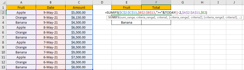
Step 1: In F2, enter the formula =SUMIFS($C$2:$C$13,$B$2:$B$13,”>=”&TODAY()-2,$A$2:$A$13,$E2).
Step 2: Press Enter after typing the formula.
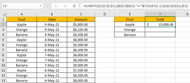
We can see $15,000.00 is returned. The format is correct. Actually, if you didn’t set the format for cell F2 before, only “15000” is returned. Before entering the formula, you need to focus on this cell, and click ‘Dollars’ icon under ‘Number’ section, and also double click on ‘Increase Decimal’ icon to add two decimal places for the returned number.
Now, let’s check the result. in column A, only cell A2, A5, A8 and A11 can meet our criteria “Fruit=Apple”, as we only sum the amounts in last 3 days, so A11 is ignored. We just need to sum amounts from C2, C5 and C8, so the total number is 5000+6000+4000=15000. The formula works correctly.
By the way, if you are confused with cell reference and range refence in the formula, we can also define range name before creating the formula. See steps below:
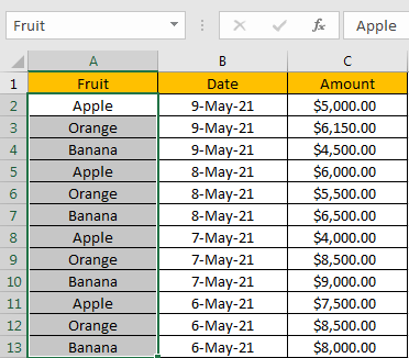
1. Select A2:A13, then in Name Box enter “Fruit”, press Enter Define reference B2:B13 as “Date”, C2:C13 as “Amount”. See screenshot below.
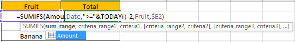
2. Then create the formula =SUMIFS(Amount,Date,”>=”&TODAY()-2,Fruit,$E2) in F2. You can enter “Amount” directly in the formula instead of selecting a range reference.
We can get the same result.
FUNCTION INTRODUCTION
SUMIFS function can be seen as SUM+IFS, it can handle multiple ‘criteria range’ and ‘criteria’ combinations.
Syntax: =SUMIFS(sum_range, criteria_range1, criteria1, [criteria_range2, criteria2], …)
For SUMIFS function, is supports wildcards like asterisk ‘*’ and question mark ‘?’, also support logical operators like “>”,”<”. If wildcards or logical operators are required, they should be enclosed into double quotes (““).
The usage of wildcards:
- An asterisk (*) means one or more characters.
- A question mark (?) means one character.
- The position of asterisk or question mark means the character(s) position relative to the entered part.
The usage of logical operators:
- “>” – greater than
- “<” – less than
- “<>” – not equal to
Today function can return current date. It doesn’t have any argument.
ALL ARGUMENTS
The formula is =SUMIFS($C$2:$C$13,$B$2:$B$13,”>=”&TODAY()-2,$A$2:$A$13,$E2). Refer to above SUMIFS function introduction, we will split it to several parts.
SUMIFS – SUM RANGE
$C$2:$C$13 is the ‘sum range’ in this case.
We add $ before row and column index to make this range as absolute references. When applying the formula to other cells, this range is locked.
Select $C$2:$C$13 from formula in the formula bar, the press F9, values in this range are expanded in an array.

SUMIFS – CRITERIA RANGE1
$B$2:$B$13 is the first criteria range. We have two criteria ranges in this instance. The first one provides date criteria.
Select $B$2:$B$13 from formula in the formula bar, the press F9, values in this range are expanded in an array.
We found that dates are converted from Date format to General format: {44325;44325;44325;44324;44324;44324;44323;44323;44323;44322;44322;44322}. Each five digits number represents a date.
SUMIFS – CRITERIA1
“>=”&TODAY()-2 is the criteria1.
As we want to sum amounts in last 3 days, except today, we only need to sum amounts on yesterday and the day before yesterday, TODAY()-2 can represent the day before yesterday, and we use “>=” to make sure this day is included in calculation.
Logical operator “>=” is quoted in “”;
Today() returns the number which can represent current date; Actually TODAY function will return current date in Date format, but we can change it to General format by selecting General in Number Format dropdown list in Number section.
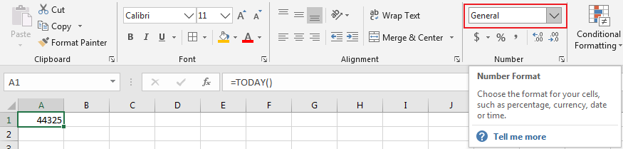
So, =TODAY()-2 is equal to 44323.
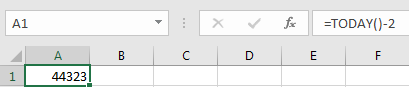
Select “>=”&TODAY()-2 from formula in the formula bar, the press F9, “>=”&44323 is displayed.
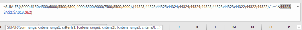
SUMIFS – CRITERIA RANGE2
$A$2:$A$13 is the second criteria range. The second one provides fruit references.
Select $A$2:$A$13 from formula in the formula bar, the press F9, values in this range are expanded in an array.
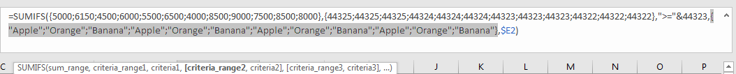
SUMIFS – CRITERIA2
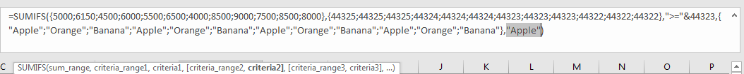
$E2 is the criteria2.
In E2, one kind of fruit “Apple” is recorded. In this case, we can omit $ actually as formula is only applied in F3 and F4 which are in the same column with F2. But if we want to copy this formula in other cells in different horizontal levels, column E will be adjusted in the formula automatically due to position changed, so we can add $ before column to lock it.
Select $E2 from formula in the formula bar, the press F9, “Apple” is displayed.
HOW THE FORMULA WORKS
After explaining each argument in the formula, now we will show you how the formula works with these arguments.
After expanding values in each range reference, in the formula bar, the formula is displayed as:
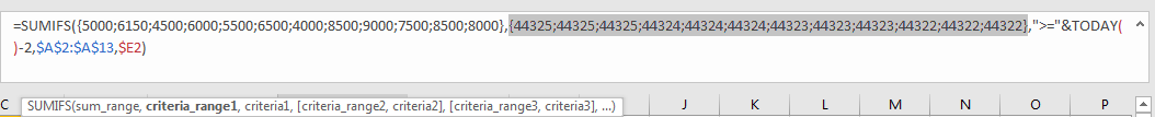
=SUMIFS({5000;6150;4500;6000;5500;6500;4000;8500;9000;7500;8500;8000},{44325;44325;44325;44324;44324;44324;44323;44323;44323;44322;44322;44322},”>=”&44323,{“Apple”;”Orange”;”Banana”;”Apple”;”Orange”;”Banana”;”Apple”;”Orange”;”Banana”;”Apple”;”Orange”;”Banana”},”Apple”)
There are two pairs of criteria range and criteria.
{44325;44325;44325;44324;44324;44324;44323;44323;44323;44322;44322;44322} – Criteria Range1
“>=”&44323 – Criteria1
And
{“Apple”;”Orange”;”Banana”;”Apple”;”Orange”;”Banana”;”Apple”;”Orange”;”Banana”;”Apple”;”Orange”;”Banana”} – Criteria Range2
“Apple” – Criteria2
If values from each criteria range are matched with the criteria, “True” will be recorded and saved, otherwise, “False” will be saved instead. So, after comparing, we can get a new criteria range:
{True;True;True;True;True;True;True;True;True;False;False;False} – after comparing with criteria1
{True;False;False;True;False;False;True;False;False;True;False;False} – after comparing with criteria2
For the following logical operation, “True” is coerced to ‘1’ and ‘False’ is coerced to ‘0’. So above two arrays are converted to below arrays which consist of numbers “1” and “0”.
{1;1;1;1;1;1;1;1;1;0;0;0} – criteria range1
{1;0;0;1;0;0;1;0;0;1;0;0} – criteria range2
As we sum range need to meet the two criteria both, so we just keep the intersection of the two arrays. If in the same position, 1 is recorded for both, keeps 1, otherwise keeps 0.
{1;0;0;1;0;0;1;0;0;0;0;0} – the intersection of the two criteria range
Now, we have below arrays:
{5000;6150;4500;6000;5500;6500;4000;8500;9000;7500;8500;8000} – sum range
{1;0;0;1;0;0;1;0;0;0;0;0} – criteria range
Elements are one-to-one matched in two arrays. Multiply the two elements in the same position in the array. Then we can get a new array.
{5000;0;0;6000;0;0;4000;0;0;0;0;0}
Add all products in above array, we get 15000.
Now, drag down the formula to fill F3 and F4. We can get total amount in last 3 days for each kind fruit properly.
SUMMARY
1. SUMIFS function can handle multiple groups of criteria ranges and criteria. Sum range is the first argument among all arguments.
2. It supports user defined range name.
3. It supports wildcard.
4. It supports logical operators.
5. TODAY function only returns current date. It has no argument.
Related Functions
- Excel SUMIF Function
The Excel SUMIF function sum the numbers in the range of cells that meet a single criteria that you specify. The syntax of the SUMIF function is as below:=SUMIF (range, criteria, [sum_range])… - Excel SUMIFS Function
The Excel SUMIFS function sum the numbers in the range of cells that meet a single or multiple criteria that you specify. The syntax of the SUMIFS function is as below:=SUMIFS (sum_range, criteria_range1, criteria1, [criteria_range2, criteria2], …)… - Excel SUM function
The Excel SUM function will adds all numbers in a range of cells and returns the sum of these values. You can add individual values, cell references or ranges in excel.The syntax of the SUM function is as below:= SUM(number1,[number2],…) - Excel TODAY function
The Excel TODAY function returns the serial number of the current date. So you can get the current system date from the TODAY function. The syntax of the TODAY function is as below:=TODAY()…