In our daily work, sometimes we may get original data in a table provided by customer or partner without arrangement, and if we want to arrange data by month or other criteria like group or others, we need to sum/extract data based on data range and then sum data and list them into another table. In this case, we need to learn how to sum data by month in columns refer to original data. Actually, we can use formula contains SUMIFS function and EOMONTH function to sum values. This tutorial will show you the way with simple descriptions and screenshots, and let you know how to use above two functions clearly.
Table of Contents
EXAMPLE:
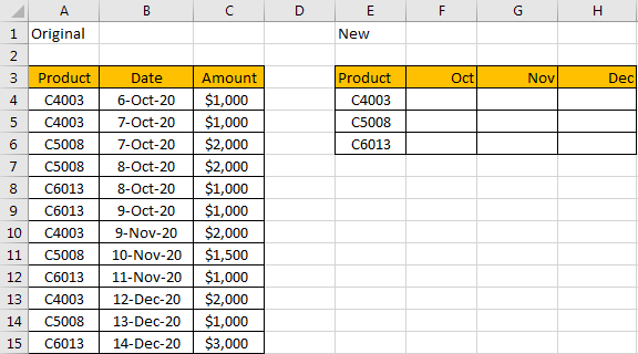
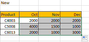
See screenshot above, we list original data in the left table, and we want to summarize them into the right table. Though we can pick data from left table and copy/past them into right table, this is troublesome and time consuming. Actually, we can apply a formula to calculate data correctly.
FORMULA:
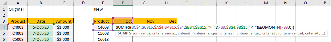
In F4 enter the formula:
=SUMIFS($C$4:$C$15,$A$4:$A$15,$E4,$B$4:$B$15,”>=”&F$3,$B$4:$B$15,”<=”&EOMONTH(F$3,0))
HOW THIS FOMULA WORKS:
This formula is based on SUMIFS function, also use EOMONTH function inside of SUMIFS.
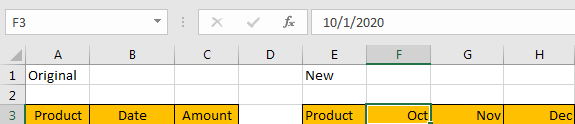
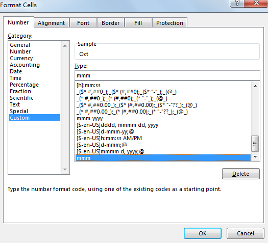
For EOMONTH function, the syntax is =EOMONTH(start_date, months), it returns the last date of a month for a specific date. For example, if date is 01/01/2020, then EOMONTH(date,0) returns 01/31/2020. In this instance, as we want to sum data belongs to October, so we need to statistic the amount for a product in a whole month. Actually, in F3, the real date is 10/1/2020, we just convert it to ‘mmm’ in customer data format.
For SUMIFS function, it sum data with multiple criteria, the syntax is =SUMIFS(sum_range, criteria_range1, criteria1, [criteria_range2, criteria2], …).
In this case, ‘sum range’ is data in ‘Amount’ list, the actual range is $C$4:$C$15, due to it is an absolute range, we don’t want to change the range when applying the formula for other cells, so we add $ before row and column number.
‘$A$4:$A$15’ is the first criteria range, and $E4 value ‘C4003’ is the first criteria, the first criteria combination ‘$A$4:$A$15,$E4’ means we want to find out product ‘C4003’ among the absolute range ‘$A$4:$A$15’. We add $ before E to lock E column, so even row is changed when coping the formula for other product in E column, the column is locked at that time.
‘$B$4:$B$15,”>=”&F$3’,’$B$4:$B$15,”<=”&EOMONTH(F$3,0)’ are criteria 2 and criteria 3. As we mentioned above, for F$3, it is 10/1/2020 in fact, so EOMONTH(F$3,0) is 10/31/2020, then we just need to find out proper date among date list ‘$B$4:$B$15’ which is greater than or equals to F$3 (10/1/2020), and less than or equals to EOMONTH(F$3,0) (10/31/2020). We add $ before row number, that’s because Oct, Nov and Dec are all listed in row 3, so we just keep row number locked in the formula.
RESULT:
Let’s see if this formula works correctly.
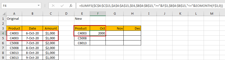
It works well. So we can drag this cell to copy the formula to other cells.
NOTES:
1.If you are consumed about the range in the formula, you can name range firstly, for example
$C$4:$C$15=Amount;
$A$4:$A$15=Product;
$B$4:$B$15=Date;
Then update formula to =SUMIFS(Amount,Product,$E4,Date,”>=”&F$3,Date,”<=”&EOMONTH(F$3,0)). It looks clearly now.
2. Oct, Nov, Dec should be actually date 10/01/2020, 11/01/2020, 12/01/2020 properly, then use Format Cells feature to convert them to proper format ‘mmm’ by Custom. Otherwise it may occur error when applying the formula due to format is improper.
Related Functions
- Excel SUMIFS Function
The Excel SUMIFS function sum the numbers in the range of cells that meet a single or multiple criteria that you specify. The syntax of the SUMIFS function is as below:=SUMIFS (sum_range, criteria_range1, criteria1, [criteria_range2, criteria2], …)…