In statistic, to create a yearly report for showing the market trend on different years, we often sum a total for different years, so based on the year’s total we can do estimation for the coming year. This scenario frequently occurs at the end of a year. If data for different dates and years are disordered in a table, how can we pick them up by year and sum total for the year correctly only by applying a formula?
To resolve this problem, we can apply Excel’s SUMIFS function and DATE function. SUMIFS function is used for sum data after filtering data based on provided criteria. Actually, it can provide multiple criteria ranges and criteria to filter data, user can sum up data based on them properly. DATE function is used for returning a date form by the given values or cell reference. Above all, we can combine the two functions into one formula to sum data by year properly.
In this article, we will show you the formula which can ‘sum data by year’ based on SUMIFS function and DATE function. To illustrate SUMIFS and DATE functions clearly, we will introduce them with their basic syntax, arguments introduction, simple usage descriptions with screenshots and explanations. In this article, we will introduce the formula from inside (DATE) to outside (SUMIFS), explain each argument in the formula, also show you the formula’s work process step by step, thus you can understand it deeply. After reading the following article, I’m sure you can learn well about SUMIFS and DATE functions, and apply them to solve your problem properly in the future.
EXAMPLE:
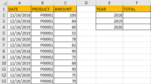
In the left table, column A lists dates in different years, column B lists product serial number P00001 and P00002, and column C lists the amount of different products on different dates and years respectively; in the right table, column E lists Year information, column F is used for recording the total amount on each Year. To calculate total amount based on year, obviously we should filter date by year, and then sum up amount values based on filtered date. For example, for cell E2 year 2018, firstly we should filter out date which is in year 2018 in column A, in this case A2, A3, A8 and A9 are filtered, then sum up C2, C3, C8 and C9. In this instance, to calculate the total amount for each year, we will apply SUMIFS and DATE function to sum data.
FORMULA APPLICATION
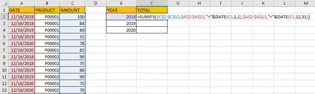
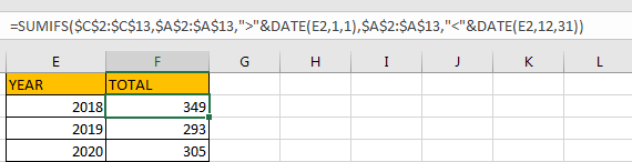
Step 1: In F2, enter the formula =SUMIFS($C$2:$C$13,$A$2:$A$13,”>”&DATE(E2,1,1),$A$2:$A$13,”<“&DATE(E2,12,31)).
Step 2: Press Enter after typing the formula.
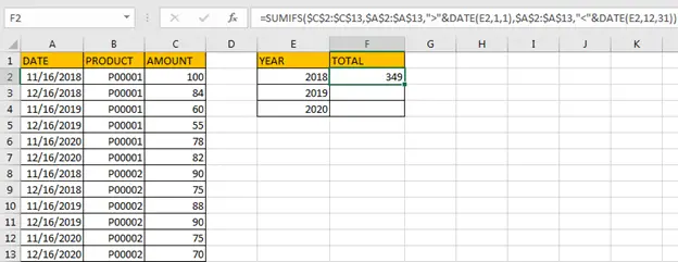
In this instance, dates in A2, A3, A8 and A9 belong to year 2018, so amounts in C2, C3, C8 and C9 should be summed. The total equals to 100+84+90+75=349. The formula works correctly.
Step 3: Apply the formula to F3 and F4. Just drag the handle down to apply this formula in F3 and F4 Verify that after dragging, the formula is updated to =SUMIFS($C$2:$C$13,$A$2:$A$13,”>”&DATE(E3,1,1),$A$2:$A$13,”<“&DATE(E3,12,31)) in F3. And value 293 is returned after pressing Enter.
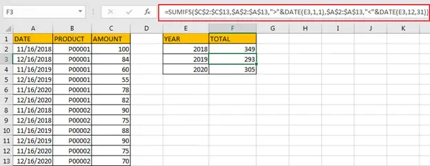
Dates in A4, A5, A10 and A11 belong to year 2019, so amounts in C4, C5, C10 and C11 should be summed. The total equals to 60+55+88+90=293. The formula still works correctly.
Step 4: Let’s check the formula in F4. The formula is =SUMIFS($C$2:$C$13,$A$2:$A$13,”>”&DATE(E4,1,1),$A$2:$A$13,”<“&DATE(E4,12,31)), total is 305. It equals to 78+82+75+70.
FUNCTIONS INTRODUCTION:
For this formula =SUMIFS($C$2:$C$13,$A$2:$A$13,”>”&DATE(E2,1,1),$A$2:$A$13,”<“&DATE(E2,12,31)), we applied two functions SUMIFS and DATE.
DATE FUNCTION:
DATE function can return a serial number that can represent a particular date if current cell format is ‘General’ or directly return a date if current cell format is ‘Date’. The syntax is
DATE(year,month,day)
All the three arguments ‘year’,’month’,’day’ are required. Please see some examples below to see the usage of DATE function.
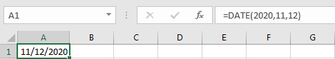
Enter =DATE(2020,11,12) in any cell, then 11/12/2020 is returned in date format.
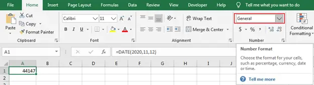
If you want to return a serial number, you can change cell format to ‘General’ via Home->Number ->General, then a number which can represents a date is displayed instead. Date 11/12/2020 is converted to 44147. On the other side, if you get 44147 after entering =DATE(2020,11,12), you can also select ‘Date’ in Number dropdown list to convert it to date. Please be aware that, in a formula DATE returns a serial number instead of date.
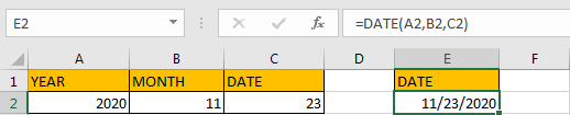
You can also save arguments in different cells, then enter cell reference into DATE function, see example below:
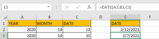
If month number is greater 12, for example 14, then 14-12=2, February of the next year will be returned. Date has the same behavior if date is greater than 31. See example below:
SUMIFS FUNCTION:
SUMIFS function can be seen as SUM+IFS, it supports multiple ‘criteria range’ and ‘criteria’ combinations.
For SUMIFS function, it has below arguments:
SUMIFS(sum_range, criteria_range1, criteria1,
[criteria_range2, criteria2]
, …). Criteria range2 and criteria2 are optional, so it still works if only one criteria range and one criterion exist. For the usage of SUMIFS function, we will split the formula to several parts, and let you know how this formula works with SUMIFS function from inside to outside.
HOW FORMULA WORKS:
=SUMIFS($C$2:$C$13,$A$2:$A$13,”>”&DATE(E2,1,1),$A$2:$A$13,”<“&DATE(E2,12,31))
In this formula:
1. ‘$C$2:$C$13’is the first argument ‘sum range’, it lists all amounts, after filtering data based on provided criteria, we pick up data from this range to sum up in the last step. As we also want to apply the formula into other cells, so we add $ before column and row to lock the range. You can see that, in former part Formula Application step#3, when copying formula to F3 and F4, this range is fixed.
In formula bar, we can convert range or executed result to actual number or array by pressing F9 in some cases. In this case, the sum range $C$2:$C$13 = {100;84;60;55;78;82;90;75;88;90;75;70}

2. ‘$A$2:$A$13’is the second argument ‘criteria_range1’. It lists dates in different years. We still add $ before column and row to lock the range.
The first criteria range A2:A13 = {43420;43450;43785;43815;44151;44181;43420;43450;43785;43815;44151;44181}.

Here we can see that date format is converted to number, each serial number represents a date. I think you are getting to know why we use DATE function in criteria argument to filter date later.
3. “>”&DATE(E2,1,1) is the argument ‘criteria1’. SUMIFS function supports logical symbols like “>”,”<” or “=”, we just need to add double quotes “” to enclose them.
DATE(E2,1,1) returns 43101. It represents date 1/1/2018, the start date in year 2018. “>”&DATE(E2,1,1) means date greater than 1/1/2018, in the formula it is “>43101”, which means number greater than 43101.

4. ‘$A$2:$A$13’is also the fourth argument ‘criteria_range2’.
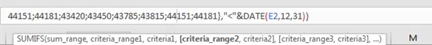
5. “<“&DATE(E2,12,31) is the argument ‘criteria2’.
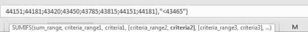
DATE(E2,12,31) returns 43465. It represents date 12/31/2018, the end date in year 2018. “<“&DATE(E2,12,31) means date less than 12/31/2018, in the formula it is “<43465”, which means number less than 43465.
Above all, the formula in E2 can be seen as below:
=SUMIFS({100;84;60;55;78;82;90;75;88;90;75;70},{43420;43450;43785;43815;44151;44181;43420;43450;43785;43815;44151;44181},”>43101″,{43420;43450;43785;43815;44151;44181;43420;43450;43785;43815;44151;44181},”<43465″)
In this formula, refer to the first group of criteria range and criteria ({43420;43450;43785;43815;44151;44181;43420;43450;43785;43815;44151;44181},”>43101″), number which is greater than 43101 will be saved as True (others are False) in the array:
{True,True,True,True,True,True,True,True,True,True,True,True }
And refer to the second group of criteria range and criteria ({43420;43450;43785;43815;44151;44181;43420;43450;43785;43815;44151;44181},”<43465″), data which is less than 43465 will be saved in the array.
{True,True,False,False,False,False,True,True,False,False,False,False}
Then compare the two arrays and keep ‘True’ for those both are True in two arrays.
{True,True,False,False,False,False,True,True,False,False,False,False}
Convert ‘True’ to ‘1’ and ‘False’ to ‘0’:
{1,1,0,0,0,0,1,1,0,0,0,0}
After filtering data by two criteria, make sure that below two arrays are vertically alignment.
Array1: {100;84;60;55;78;82;90;75;88;90;75;70} – sum range
Array2: {1,1,0,0,0,0,1,1,0,0,0,0}) – criteria
Keep current value in array1 if its corresponding value is 1 in array2, otherwise value is changed to 0. You can also think value in array1 multiplies the corresponding value in array2. Thus, we can get another array:
Array3: {100;84;0;0;0;0;90;75;0;0;0;0} – sum range
Sum data in array3, 100+84+90+75=349.
The formula work process is the same for F3 and F4.
Related Functions
- Excel DATE function
The Excel DATE function returns the serial number for a date.The syntax of the DATE function is as below:= DATE (year, month, day)… - Excel YEAR function
The Excel YEAR function returns a four-digit year from a given date value, the year is returned as an integer ranging from 1900 to 9999. The syntax of the YEAR function is as below:=YEAR (serial_number)…