For a set of data, if we want to sum data for a range between two numbers, we need to sum data based on ‘> criteria A and < criteria B’, so there are two criteria here. In our daily work, this case frequently occurs when calculating total score or total amount for a range.

To resolve this problem, we can apply excel SUMIFS functions. SUMIFS function can provide multiple criteria ranges and criteria arguments, user can sum up data based on these criteria. To sum data between two numbers, the two numbers are two important arguments. So through providing criteria ranges, criteria and sum range, we can filter out data between two numbers and then sum them up.

In this article, we will show you the formula which can ‘sum data if between number A and number B’ based on SUMIFS function. To illustrate SUMIFS function clearly, we will introduce it with basic syntax, argument introduction, simple usage description with screenshots and explanations. In this article, we will introduce the formula work process step by step, explain each argument in the formula, thus you can understand it deeply. After reading the following article, I’m sure you can learn well about SUMIFS function, and apply it to solve your problem properly in the future.

EXAMPLE:

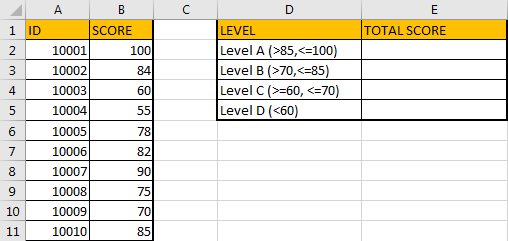
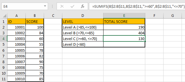
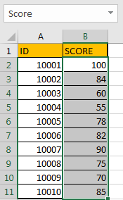
In the left table, column B lists all scores; in the right table, column D lists the score range for each level, column E is used for recording the total score for each level, what we want to do is sum data based on each level. We can refer to the description of each level to sum data. For example, for level A, the range is ‘>85 and <=100’, so we need to filter data which is between 85 and 100, then sum up. In this instance, we will apply SUMIFS to sum data.

FORMULA – SUMIFS FUNCTION

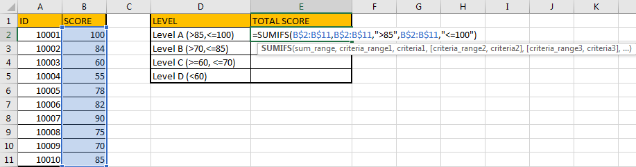
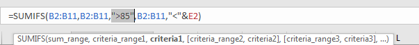
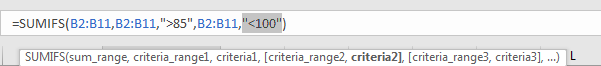
Step1: In E2, enter the formula =SUMIFS(B$2:B$11,B$2:B$11,”>85″,B$2:B$11,”<=100″). “>85” and “<=100” are the two criteria for level A.

Step2: Press Enter after typing the formula.

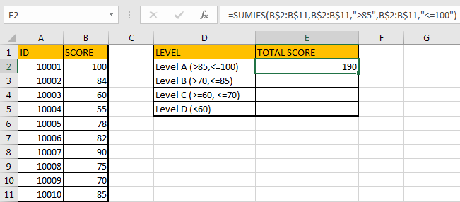
In this instance, only ID 10001 with score 100 and ID 10007 with score 90 match the criteria, so the total score is 100+90=190. The formula works correctly.

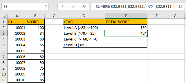
Step3: Based on above formula, we enter the formula =SUMIFS(B$2:B$11,B$2:B$11,”>70″,B$2:B$11,”<=85″) in E3. It equals to 84+78+82+75+85=404.

Step4: Enter =SUMIFS(B$2:B$11,B$2:B$11,”>=60″,B$2:B$11,”<=70″) in E4. We can get 130 correctly.

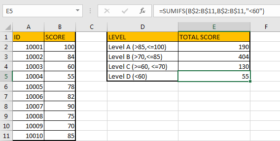
Step5: In E5, enter the formula =SUMIFS(B$2:B$11,B$2:B$11,”<60″). In this formula, there is only one group of criteria range and criteria, it still works well.

HOW FORMULA WORKS:

SUMIFS function can be seen as SUM+IFS, it supports multiple ‘criteria range’ and ‘criteria’ combinations.

For SUMIFS function, it has below arguments:

SUMIFS(sum_range, criteria_range1, criteria1, [criteria_range2, criteria2], …). Criteria range2 and criteria2 are optional, so it still works if only one criteria range and one criterion exist.

In our instance, ‘B2:B11’ is the sum range and also the criteria range, it lists all scores, we want sum scores in this column which match the two criteria (>criteria1, <criteria2). If we want to apply the formula directly into other cells, we can add $ before column and row to lock the range per your request. Then when copying formula to other cells, this range is fixed.

The sum range B2:B11 = {100;84;60;55;78;82;90;75;70;85}

The first criteria range B2:B11 = {100;84;60;55;78;82;90;75;70;85}.

Criteria1 is “>85”. As for level A, data is greater than 85 and less than or equals to 100, so in criteria1, we enter “>85”. We can see that SUMIFS function supports logical operators like ‘>’,’<’ and ‘=’. We enclose these logical operators and entered texts like ‘85’ into double quotes (““).

The second criteria range B2:B11 = {100;84;60;55;78;82;90;75;70;85}.

Criteria2 is “<=100”.

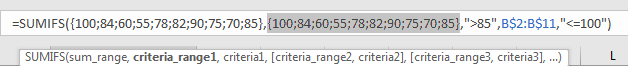
Above all, the formula in E2 can be seen as below:

=SUMIFS({100;84;60;55;78;82;90;75;70;85},{100;84;60;55;78;82;90;75;70;85},”>85″,{100;84;60;55;78;82;90;75;70;85},”<=100″)

In this formula, refer to the first group ({100;84;60;55;78;82;90;75;70;85},”>85″), data which is greater than 35 will be saved as True (others are False) in an array:

{True,False,False,False,False,False,True,False,False,False}

And refer to the second group ({100;84;60;55;78;82;90;75;70;85},”<=100″), data which is less than or equals to 100 will be saved in another array.

{True,True,True,True,True,True,True,True,True,True}

SUMIFS function will find out the intersection of the two arrays:

{True,False,False,False,False,False,True,False,False,False}

Convert to 1 (True) and 0 (False):

{1,0,0,0,0,1,0,0,0}

And then locate the data in sum range based on the intersection:

{100,0,0,0,0,90,0,0,0} 

And finally sum up filtered data in sum range:

100+90=190.

ANOTHER EXAMPLE:

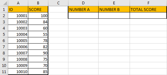
In this example, number A and number B are not fixed, so to calculate total score for a range between two dynamic numbers, we can still use SUMIFS function, but for criteria part, we can enter cell reference instead of enter text. Thus, when changing the numbers, the total score is recalculated based on the two numbers properly without updating the formula.

FORMULA – SUMIFS FUNCTION 2

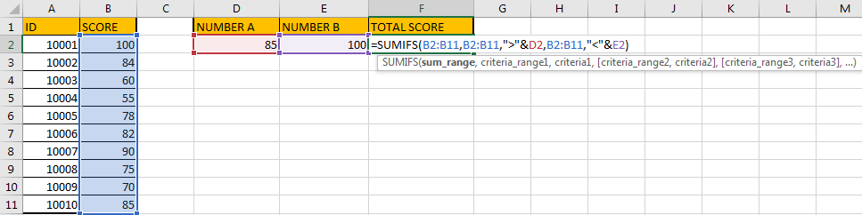
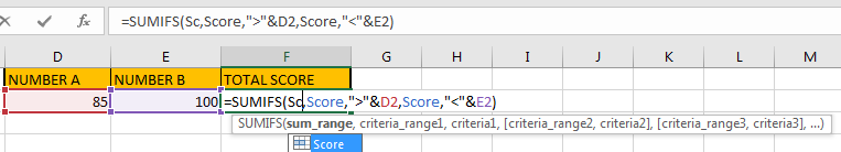
Step1: In E2 enter the formula =SUMIFS(B2:B11,B2:B11,”>”&D2,B2:B11,”<“&E2).

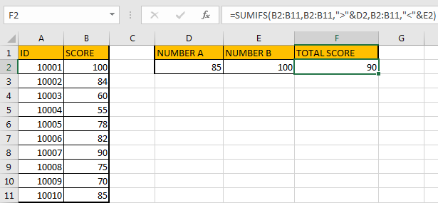
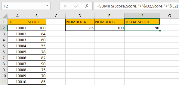
Step2: Press Enter and get the returned value.

HOW FORMULA WORKS:

In this formula, compare with the former one, the difference is we enter cell reference instead of entering real number in criteria. We can change the values in number A and number B, so the total score is updated based on the two cells dynamically.

For criteria1, it is “>”&D2, we still use double quotes (“”) to enclose logical operators or texts, D2 provides the number, symbol & is used for connecting logical operator and cell reference. You can also change the logical operator to “>=” per your request. In D2, the value is 85, it is equivalent to “>85” in former example.

For criteria2, it is “<“&E2, it is equivalent to “<100”.

Above all, the formula in E2 can be seen as below:

=SUMIFS({100;84;60;55;78;82;90;75;70;85},{100;84;60;55;78;82;90;75;70;85},">85",{100;84;60;55;78;82;90;75;70;85},"<100")

You can see that the two formulas are the same after converting each argument to real number or number arrays. The work processes are the same.

By the say, if you are confused of using cell reference, you can define sum range or criteria range with proper name firstly, then apply range name in your formula. See example below:

Step1: select B2:B11, then enter the range name. We name it ‘Score’.

Step2: When entering ‘Sc’ in formula, you may find user defined ‘Score’ is loaded.

Step3: After entering the complete formula, proper value is returned.

SUMMARY:

1. In this instance, we must make sure that based on the two criteria, two criteria ranges have intersection, otherwise “0” is returned, no error message pops up.
2. You can enter actual numbers or cell reference into criteria arguments based on the real situation.
3. SUMIFS is frequently used in sum up data based on multiple criteria. You can take this function into consideration when meeting the similar cases.

Video: Sum Data if Between Two Numbers

This Excel video tutorial where we’ll delve into the effective method of summing data falling between two numbers.

Related Functions

• Excel SUMIFS Function
  The Excel SUMIFS function sum the numbers in the range of cells that meet a single or multiple criteria that you specify. The syntax of the SUMIFS function is as below:=SUMIFS (sum_range, criteria_range1, criteria1, [criteria_range2, criteria2], …)…