For a set of data, sometimes we may need to sum some of them based on criteria ‘if begins with/end with/contains’ ** characters. In our daily work, this case frequently occurs when calculating total for one or more items among a lot of different type of items.
To resolve this problem, we can apply excel SUMIF and SUMIFS functions. For these two functions, ‘criteria’ is an important argument, so through providing proper criteria range, criteria and sum range, we can filter out data matches the entered criteria and then sum data based on the filtered data.
In this article, we will show you the formula which can ‘sum data if begins/end with or contains ** characters’ based on SUMIF or SUMIFS functions. These two functions are frequently used in sum data with ‘Criteria’. We will introduce above two functions with simple examples, descriptions, screenshots and explanations in this article, and also show you the usage of them. As the two functions look similar, we will also introduce the difference between them. At last, we will let you know the function/formula workflow step by step clearly. After reading the following article, I’m sure you can have a simple understanding of SUMIF or SUMIFS functions.
EXAMPLE:
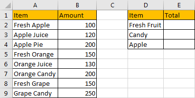
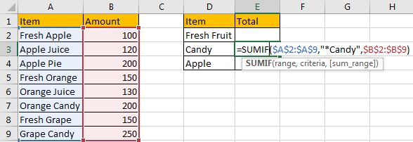
In above table, the first item is ‘Fresh Fruit’, so we can sum data based on criteria in A column which begins with ‘Fresh’; for the second item ‘Candy’, we can see ‘Orange Candy’, ’Grape Candy’ are end with ‘Candy’, so we can sum data based on criteria ends with ‘Candy’; for the third item ‘Apple’, ‘Fresh Apple’, ’Apple Juice’ and ‘Apple Pie’ contain ‘Apple’, so we can sum data based on criteria contains ‘Apple’. We will apply formula contains SUMIF or SUMIFS to sum data refer to above three scenarios.
FORMULA – SUMIF FUNCTION
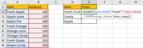
Step 1: In E2, enter the formula =SUMIF($A$2:$A$9,”Fresh*”,$B$2:$B$9). ‘Fresh’ is the criteria, we add an asterisk (*) after ‘Fresh’, it means one or more characters exist following word ‘Fresh’.
Step 2: Press Enter after typing the formula.
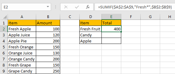
‘Fresh Apple:100’+’Fresh Orange:150’+’Fresh Grape:150’=400. We get 400 by applying the formula. So the formula works properly.
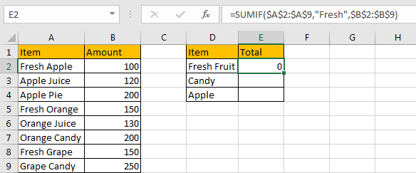
If we omit (*) in criteria ‘Fresh*’, 0 is returned as there is no criteria exactly equals to ‘Fresh’.
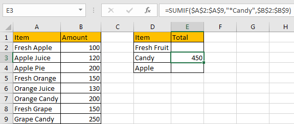
Step 3: In E3, enter the formula =SUMIF($A$2:$A$9,”*Candy”,$B$2:$B$9). ‘Candy’ is the criteria, we add an asterisk (*) before ‘Candy’, it means one or more characters exist before word ‘Fresh’.
Step 4: Press Enter after typing the formula. ‘Orange Candy:200’+’Grape Candy:250’=450.
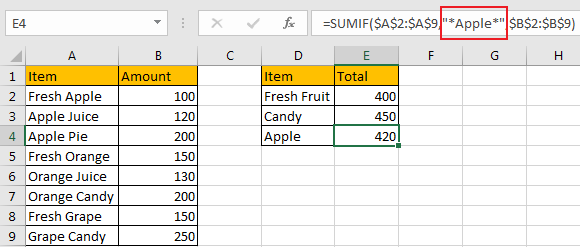
Step 5: In E4, enter the formula =SUMIF($A$2:$A$9,”*Apple*”,$B$2:$B$9). ‘Apple’ is the criteria, we add asterisk (*) before and after ‘Apple’, then all contents contain ‘Apple’ are filtered, amounts for filtered ‘Apple’ are summed.
HOW FORMULA WORKS:
For SUMIF function, the syntax as below:
SUMIF(range, criteria, [sum range])
The first argument ‘range’ is the criteria range, in our instance, for three items, the criteria range is the same range ‘$A$2:$A$9’, we add $ before range A2:A9 to lock this range, so when copy this formula to other cells, reference A2:A9 is will not be auto changed.
The second argument ‘criteria’ is the criteria we sum data based on. In above applied formulas, the criteria are “Fresh*”, “*Candy” and “*Apple*” respectively. It reflects that SUMIF function can support wildcards in its formula, and it requires to add double quotes (““) to enclose wildcards or texts. An asterisk (*) means one or more characters. A question mark (?) means one character. The position of asterisk or question mark means the character(s) position relative to the entered part.
The third argument ‘sum range’ lists values can be used for sum. Through the first two arguments, we can filter data in criteria range based on the criteria, after filtering, amount for the filtered data are summed.
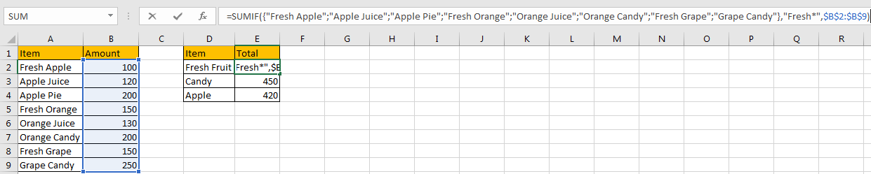
This formula can be seen like this:
=SUMIF({“Fresh Apple”;”Apple Juice”;”Apple Pie”;”Fresh Orange”;”Orange Juice”;”Orange Candy”;”Fresh Grape”;”Grape Candy”},”Fresh*”,{100;120;200;150;130;200;150;250})
If texts in criteria range begins with ‘Fresh’, then the result is TRUE, otherwise the result is FALSE. So after comparing, the result can be seen as {TRUE,FALSE,FALSE,TRUE,FALSE,FALSE,TRUE,FALSE}. So the formula is equivalent to {1,0,0,1,0,0,1,0}*{100;120;200;150;130;200;150;250}={100,0,0,150,0,0,150,0}. SUM data in this array, we can get 400. In E2 the result is 400 as well.
Through above analysis process, we can also analysis the working process for the formulas in E3 and E4. They are exactly the same because we only apply SUMIF function here.
FORMULA – SUMIFS FUNCTION
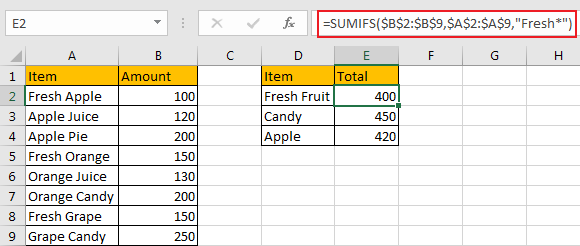
Step 1: In E2 enter the formula =SUMIFS($B$2:$B$9,$A$2:$A$9,”Fresh*”).
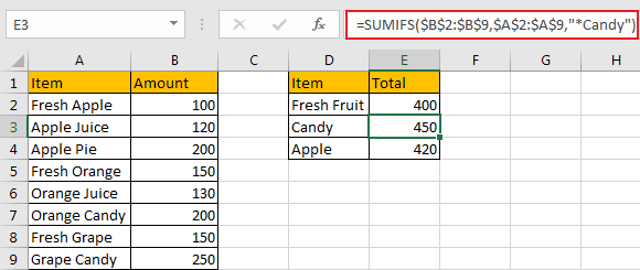
Step 2: In E3 enter the formula =SUMIFS($B$2:$B$9,$A$2:$A$9,”*Candy”).
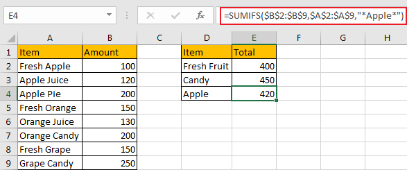
Step 3: In E4 enter the formula =SUMIFS($B$2:$B$9,$A$2:$A$9,”*Apple*”).
After pressing Enter, we can see we get the same results by applying SUMIF function.
HOW FORMULA WORKS:
SUMIFS function looks similar to SUMIF, it only has an extra ‘S’ than SUMIF. SUMIF function can be seen as SUM+IF, it has only one group of ‘criteria range’ and ‘criteria’, but SUMIFS function can be seen SUM+ IFS, it can have multiple ‘criteria range’ and ‘criteria’ combinations.
For SUMIFS function, it has below arguments:
SUMIFS(sum_range, criteria_range1, criteria1, [criteria_range2, criteria2], …).
In our instance, $B$2:$B$9 is the sum range, it provides values to do sum calculation. If we want to set it as an absolute range, we can add $ before column and row to lock the range. Then when copying formula to other cells, this range is fixed.
$B$2:$B$9 =({100;120;200;150;130;200;150;250}
![]()
$A$2:$A$9 is the criteria range, in this case we have only one criteria range.
{“Fresh Apple”;”Apple Juice”;”Apple Pie”;”Fresh Orange”;”Orange Juice”;”Orange Candy”;”Fresh Grape”;”Grape Candy”}
![]()
“Fresh*”, “*Candy” and “*Apple*” are criteria for the three formulas respectively. We compare each value in criteria range $A$2:$A$9 with the entered text, if the entered text can be found with correct position, corresponding amount value in sum range $B$2:$B$9 will be summed. By this way, we get total amount based on the criteria. Above all, the formula in E4 can be seen as below:
=SUMIFS({100;120;200;150;130;200;150;250},{“Fresh Apple”;”Apple Juice”;”Apple Pie”;”Fresh Orange”;”Orange Juice”;”Orange Candy”;”Fresh Grape”;”Grape Candy”},”*Apple*”)
For the following steps, you can refer to SUMIF function working process.
SUMMARY:
- SUMIF function has only one group of criteria range and criteria, sum range is listed in the last position in the formula.
- SUMIFS function has multiple groups of criteria ranges and criteria, sum range is listed in the first position of the formula.
- They are frequently used in summing data based on criteria.
Related Functions
- Excel SUMIF Function
The Excel SUMIF function sum the numbers in the range of cells that meet a single criteria that you specify. The syntax of the SUMIF function is as below:=SUMIF (range, criteria, [sum_range])… - Excel SUMIFS Function
The Excel SUMIFS function sum the numbers in the range of cells that meet a single or multiple criteria that you specify. The syntax of the SUMIFS function is as below:=SUMIFS (sum_range, criteria_range1, criteria1, [criteria_range2, criteria2], …)…