In statistic report, we often statistic data for a certain date range. Sometimes we can use an exact week number instead of entering a start date and an end date as a period to statistic data.
For example, to sum data by week 1, that means we only need to calculate data belongs to week 1 other than a fixed date range with start date and end date. In this case, if week number is not provided in original data table, we need to use WEEKNUM function to get week number for entered date firstly, then we can use a formula contains SUMIFS function to sum data by this week properly. This tutorial will show you ‘sum by week number’ with simple descriptions, screenshots and explanations, and we will let you know how WEEKNUM and SUMIFS functions work, how to set parameters in the formula, you can learn sum data per your requirement clearly by yourself, and finally, you can work well with these functions in your daily work.
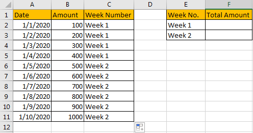
EXAMPLE:
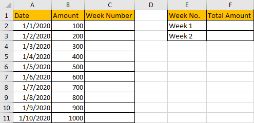
FORMULA:
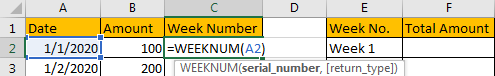
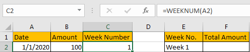
As we need to sum data by week number, first of all, we need to get week number for all entered data in ‘Date’ list. So, in C2, enter the formula =WEEKNUM(A2).
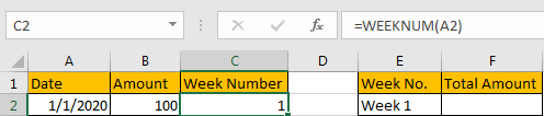
After clicking Enter, we get ‘1’ as the formula result.
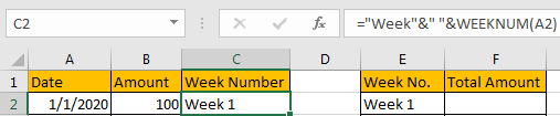
As we enter ‘Week 1’ as criteria in ‘Week No.’ column, so we need to display ‘Week + No.’ in ‘Week Number’ column as well, otherwise we cannot apply formula properly. Update previous formula to =”Week”&” “&WEEKNUM(A2). Then we get ‘Week 1’ properly.
Drag down the cell to copy the formula. Then we can get all week numbers for entered dates.
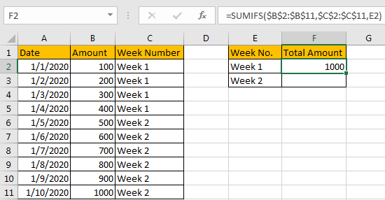
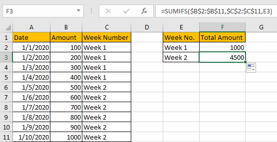
Now, we have all week numbers, we can apply SUMIFS function to sum data per week number criteria properly. In F1 enter the formula =SUMIFS($B$2:$B$11,$C$2:$C$11,E2). After clicking Enter, we can get correct total amount 1000.
HOW THIS FORMULA WORKS:
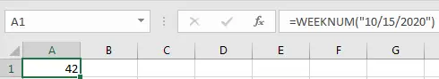
Firstly, we applied WEEKNUM function in this instance. WEEKNUM function can returns week number for the entered date. You can enter a date within double quote in the function. For example, enter =WEEKNUM(“10/15/2020”), click Enter, we will get 42. That means 10/15/2020 belongs to week 42 in this year.
We can also select a cell number directly when applying this function. In this instance, we can get correct week number after applying the formula.
Then we use SUMIFS function =SUMIFS($B$2:$B$11,$C$2:$C$11,E2) to sum data. For SUMIFS function, it sum data with multiple criteria, the syntax is =SUMIFS(sum_range, criteria_range1, criteria1, [criteria_range2, criteria2], …).
In this case, $B$2:$B$11 is the sum range, it provides values to sum, as it is an absolute range in this case, so we add $ before row and column number to lock the range, so when copying formula to other cells, this range is fixed, user doesn’t need to adjust the sum range any more.
$C$2:$C$11 is the criteria range, it provides all week numbers, it is an absolute range in this case as well, so we add $ before row and column number; as we want to find out week number from this range matches to week 1, so we must find out all week 1 in ‘Week Number’ column, above all, the last parameter in the formula is E2: Week 1.
RESULT:
Let’s check if the formula works well for week 1 and week 2.
EXAMPLE 2:
This instance is a bit more complex then former instance. See screenshot below:
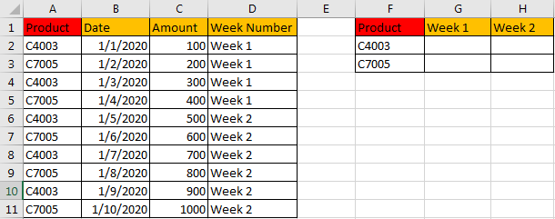
We add ‘Product’ into original data table and destination table. In above screenshot we can see that week numbers are already calculated properly by WEEKNUM function refer to former instance. In this instance, we just need to update formula which is based on SUMIFS function.
FORMULA:
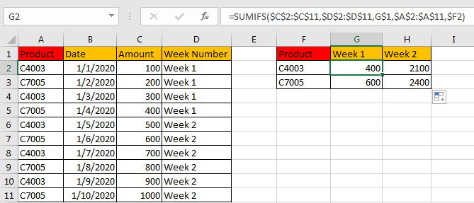
In G1 enter the formula =SUMIFS($C$2:$C$11,$D$2:$D$11,G$1,$A$2:$A$11,$F2).
HOW THIS FORMULA WORKS:
Compare with former formula =SUMIFS($B$2:$B$11,$C$2:$C$11,E2), SUMIFS function has two criteria ranges and two criteria.
The first criteria range: $D$2:$D$11 (Week Number), the matching criteria is G$1 (Week 1);
The second criteria range: $A$2:$A$11 (Product), the matching criteria is $F2 (C4003).
There is no priority for the two groups of criteria range and criteria, you can change the order if you like, formula =SUMIFS($C$2:$C$11,$A$2:$A$11,$F2,$D$2:$D$11,G$1) also works.
Unlike the criteria ‘E2’ in example 1 (when copying the formula to next cell, E2 is updated to E3 automatically), we add $ in criteria ‘G$1’ before ‘1’ to lock row number because week1 is in G1 and week2 is in H1, the row number is fixed, so row number should be kept in formula and only column can be updated automatically when copying the formula to other cells. For example, if $ is not added, when applying the formula for cell G2, the criteria will be changed from G1 to G2, the criteria is not ‘Week 1’ anymore, the formula is executed improperly.
Besides, we also add $ before ‘F’ in criteria ‘$F2’ to lock ‘F’ column with similar reason, so even we copy the formula to H2, the criteria is still F2 in the formula and will not be changed to G2 in the case that $ is not added.
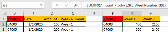
RESULT:
Let’s see if this formula works correctly. Obviously, it works well.
NOTES:
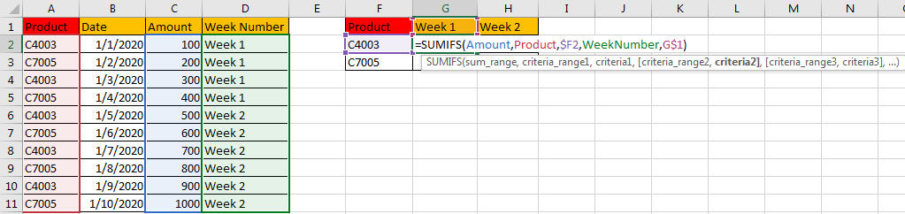
If you are confused of the sum range and criteria range in the formula, you can also name range firstly, for example
$C$2:$C$11=Amount;
$D$2:$D$11=WeekNumber;
$A$2:$A$11=Product.
To name range, just select the whole range (for example A2:A11, ignore the header), and enter name in name box (for example ‘Product’). Please be aware that there should be NO space in name.
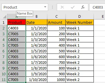
Then update formula to =SUMIFS(Amount,Product,$F2,WeekNumber,G$1). It looks clearly now.
Check the result for the formula. It works well.
Related Functions
- Excel WEEKNUM function
The Excel WEEKNUM function returns the week number of a specific date, and the returned value is ranging from 1 to 53.The syntax of the WEEKNUM function is as below:=WEEKNUM (serial_number,[return_type])… - Excel SUMIFS Function
The Excel SUMIFS function sum the numbers in the range of cells that meet a single or multiple criteria that you specify. The syntax of the SUMIFS function is as below:=SUMIFS (sum_range, criteria_range1, criteria1, [criteria_range2, criteria2], …)…